
BIOL-430 · Lesson 7 of 12 · 24 min
Measuring biodiversity in the field
Biodiversity sounds simple to measure: walk around, list the species, count them. In practice, the number on the list depends on how hard you looked, where, when and with what skill; two sites can have the same species richness and almost no species in common; and much of what matters about a community, such as how many pollinators or nitrogen fixers it has, is not captured by a species count. BIOL-367 introduced diversity indices, Hill numbers, rarefaction and the Chao1 estimator for a single sample of individuals. This lesson focuses on the field side: designing biodiversity surveys, sample-based accumulation and incidence-based estimators, beta diversity and its decomposition, functional and phylogenetic diversity, and new tools such as bioacoustics and community science.
Effort, completeness and the species list
Every species list is incomplete. Common species appear early in a survey, rare ones trickle in as effort accumulates, and some are never found. Plotting the cumulative number of species against effort, whether hours searched, quadrats sampled or individuals counted, gives a species accumulation curve. Its shape tells you about completeness: a curve still climbing steeply means many species remain undetected; one that has flattened means further effort will add few. Comparing richness between sites or treatments is only fair when effort is standardized or when the comparison is made at a common level of coverage, the proportion of the community's individuals that belong to species already detected.
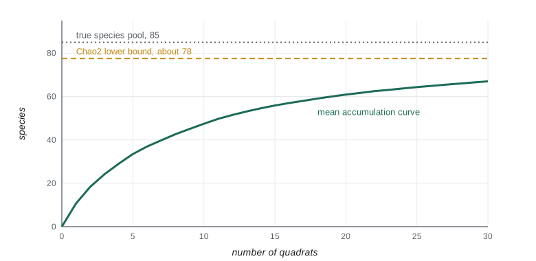
Field surveys often record incidence, the presence or absence of each species in each of several sampling units such as quadrats, point counts or pitfall traps, rather than counts of individuals. Sample-based accumulation curves, built by adding sampling units in random order and averaging over many orders, are the incidence analogue of rarefaction. Plant surveys in the grazing study use 30 quadrats of 1 square metre along wetland edges at each wetland; the species recorded in each quadrat form an incidence matrix.
Incidence-based richness estimators
Chao2 is the incidence counterpart of Chao1. It uses \(Q_1\), the number of species found in exactly one sampling unit (uniques), and \(Q_2\), the number found in exactly two (duplicates). With \(m\) sampling units and \(S_{obs}\) species observed,
The logic is the same as for Chao1: if many species are uniques, many more are probably still unseen. Chao2 is a lower bound for true richness, not an exact estimate, and is most reliable when sampling units are numerous and randomly placed. The incidence-based coverage estimator (ICE) and jackknife estimators are alternatives; all perform badly when sampling is very incomplete, and none can find species that the method cannot detect at all, such as plants that are dormant in a dry year.
# Sample-based accumulation and Chao2 for wetland-edge plants in 30 quadrats (synthetic).
import numpy as np
rng = np.random.default_rng(73)
S_true, m = 85, 30
freq = np.sort(rng.beta(0.8, 5.0, S_true))[::-1]        # per-quadrat occurrence probabilities
inc = rng.uniform(size=(m, S_true)) < freq                # quadrats x species incidence
seen = inc.any(0); S_obs = seen.sum()
q = inc.sum(0)
Q1, Q2 = (q == 1).sum(), (q == 2).sum()
chao2 = S_obs + (m - 1) / m * Q1**2 / (2 * Q2)
curve = np.zeros(m)
for _ in range(500):
    order = rng.permutation(m)
    curve += np.array([inc[order[:k + 1]].any(0).sum() for k in range(m)])
curve /= 500
print("mean species after 1, 5, 10, 20, 30 quadrats:", " ".join(f"{curve[k - 1]:.1f}" for k in (1, 5, 10, 20, 30)))
print(f"observed {S_obs}, uniques Q1 = {Q1}, duplicates Q2 = {Q2}, Chao2 = {chao2:.1f} (true pool {S_true})")
print(f"species added by the last 10 quadrats: {curve[-1] - curve[19]:.1f}")mean species after 1, 5, 10, 20, 30 quadrats: 10.5 33.2 47.6 60.9 67.0 observed 67, uniques Q1 = 14, duplicates Q2 = 9, Chao2 = 77.5 (true pool 85) species added by the last 10 quadrats: 6.1
After 30 quadrats the curve is still rising, adding about six species over the last ten quadrats, and Chao2 suggests about ten species remain undetected. Even so, it falls short of the true pool of 85, because the rarest species in this invented community occur in so few quadrats that they leave almost no trace in the uniques and duplicates; this is exactly why Chao2 is called a lower bound.
Alpha, beta and gamma diversity
Whittaker distinguished diversity within a site (alpha), among sites (beta) and over a whole region (gamma). In his multiplicative formulation, \(\beta = \gamma / \bar{\alpha}\): if each wetland edge holds 25 species on average and the station as a whole holds 100, beta diversity is 4, meaning the landscape holds as many species as four completely distinct wetlands would. Beta diversity matters for conservation and management because it describes how much each site adds. Two grazing regimes could produce identical alpha diversity at each wetland but very different beta diversity, if one homogenizes communities across the landscape and the other keeps them distinct.
Pairwise dissimilarity indices compare two sites. For incidence data, with \(a\) species shared and \(b\) and \(c\) unique to each site, the Sørensen dissimilarity is \((b + c)/(2a + b + c)\) and the Jaccard dissimilarity is \((b + c)/(a + b + c)\). Baselga (2010) showed that Sørensen dissimilarity can be split into turnover, the replacement of species by others, measured by the Simpson dissimilarity \(\min(b, c)/(a + \min(b, c))\), and nestedness, the loss of species so that one site's list is a subset of the other's. The distinction matters: grazing that strips sensitive species from wetland edges produces nestedness, whereas a shift from wet-meadow to upland species produces turnover.
# Beta diversity between a fenced and a grazed wetland edge: Sorensen, turnover and nestedness.
fenced = set("Carex atherodes|Carex aquatilis|Scolochloa festucacea|Typha latifolia|Glyceria grandis|"
             "Calamagrostis canadensis|Mentha arvensis|Stachys pilosa|Sium suave|Rumex occidentalis|"
             "Beckmannia syzigachne|Hordeum jubatum|Poa palustris|Juncus balticus|Epilobium ciliatum".split("|"))
grazed = set("Carex atherodes|Typha latifolia|Hordeum jubatum|Poa pratensis|Taraxacum officinale|"
             "Juncus balticus|Beckmannia syzigachne|Polygonum aviculare|Plantago major|Puccinellia nuttalliana".split("|"))
a = len(fenced & grazed); b = len(fenced - grazed); c = len(grazed - fenced)
sor = (b + c) / (2 * a + b + c)
sim = min(b, c) / (a + min(b, c))
print(f"shared a = {a}, only fenced b = {b}, only grazed c = {c}")
print(f"Sorensen dissimilarity = {sor:.2f}: turnover (Simpson) = {sim:.2f} + nestedness = {sor - sim:.2f}")
print("species only in the grazed edge:", ", ".join(sorted(grazed - fenced)))shared a = 5, only fenced b = 10, only grazed c = 5 Sorensen dissimilarity = 0.60: turnover (Simpson) = 0.50 + nestedness = 0.10 species only in the grazed edge: Plantago major, Poa pratensis, Polygonum aviculare, Puccinellia nuttalliana, Taraxacum officinale
Beyond species counts: functional and phylogenetic diversity
Species richness treats every species as equal and different from every other by the same amount. Functional diversity instead considers traits, such as plant height, leaf nitrogen, root depth, seed mass and growth form, or for animals body size, diet and foraging guild. Simple measures include the community-weighted mean of a trait, the average trait value weighted by each species' abundance, and functional richness or dispersion, the volume or spread of species in trait space. Traits link communities to processes: a shift toward short, grazing-tolerant, rosette-forming plants signals reduced nest cover and possibly lower carbon storage, whatever happens to species counts.
Phylogenetic diversity, introduced by Faith in 1992, sums the branch lengths of the evolutionary tree connecting the species in a community, so a community of distantly related species scores higher than one of close relatives. It captures evolutionary history that might be lost and, because related species often share traits, it can stand in for unmeasured functional differences. Both functional and phylogenetic measures depend on good trait databases and phylogenies, which are increasingly available, such as the TRY plant trait database.
# Community-weighted mean plant height in fenced and grazed edges (synthetic cover data).
heights = {'Carex atherodes': 90, 'Typha latifolia': 180, 'Hordeum jubatum': 45, 'Poa pratensis': 40,
           'Taraxacum officinale': 15, 'Scolochloa festucacea': 120, 'Plantago major': 10, 'Juncus balticus': 50}
cover = {   # percent cover by species
    'fenced': {'Carex atherodes': 30, 'Typha latifolia': 18, 'Scolochloa festucacea': 22, 'Hordeum jubatum': 8, 'Juncus balticus': 6},
    'grazed': {'Carex atherodes': 14, 'Typha latifolia': 6, 'Hordeum jubatum': 20, 'Poa pratensis': 18, 'Taraxacum officinale': 9,
               'Plantago major': 7, 'Juncus balticus': 10},
}
for site, cv in cover.items():
    tot = sum(cv.values())
    cwm = sum(heights[s] * c for s, c in cv.items()) / tot
print(f"{site}: {len(cv)} species, total cover {tot}%, community-weighted mean height {cwm:.0f} cm")fenced: 5 species, total cover 84%, community-weighted mean height 110 cm grazed: 7 species, total cover 84%, community-weighted mean height 56 cm
The example shows why richness alone can mislead. The grazed edge has more species, many of them introduced or disturbance-tolerant, while the fenced edge has fewer but taller species that provide the cover ducks and sparrows need. A management evaluation that reported only richness would reach the wrong conclusion.
| Measure | What it captures | Field data needed | Caution |
|---|---|---|---|
| Species richness | Number of species | Species list with standardized effort | Depends strongly on effort and detection |
| Chao2 or jackknife | Lower bound on total richness | Incidence in many sampling units | Unreliable when sampling is very incomplete |
| Hill numbers (from BIOL-367) | Diversity weighting rare to common species | Abundances or cover | Report several orders, with coverage |
| Sorensen and Jaccard | Compositional difference between sites | Incidence at each site | Sensitive to undersampling |
| Turnover and nestedness | Replacement versus loss of species | Incidence at each site | Interpretation depends on scale |
| Community-weighted mean | Average trait of the community | Abundances plus trait values | Traits vary within species too |
| Phylogenetic diversity | Evolutionary history represented | Species list plus phylogeny | Depends on tree quality |
Bioacoustics
Autonomous recording units, weatherproof recorders that can run unattended for weeks, have changed bird, frog and bat surveys. They record at scheduled times, such as dawn and dusk, removing observer differences and allowing far more sampling than a crew could do in person. Recordings can be listened to by trained people, scanned by automated classifiers such as BirdNET, or summarized with acoustic indices, which measure properties of the soundscape such as the variability of intensity across frequencies (the acoustic complexity index) or the evenness of sound across frequency bands. Indices are quick but loosely related to species richness and easily confounded by wind, rain, insects and traffic, so they are best calibrated against species identifications. In Canada, the Bioacoustic Unit and the WildTrax platform, developed at the University of Alberta and the Alberta Biodiversity Monitoring Institute, host millions of recordings for processing and sharing.
Community science
Volunteers contribute much of the biodiversity data in North America. eBird, run by the Cornell Lab of Ornithology, holds well over a billion bird observations worldwide; iNaturalist links photos to identifications by a community of naturalists; the Christmas Bird Count, run by the National Audubon Society with Birds Canada, has run since 1900; and the Breeding Bird Survey depends on volunteer observers. In Canada, Birds Canada coordinates provincial breeding bird atlases and NatureCounts, and the Alberta Biodiversity Monitoring Institute runs a province-wide systematic monitoring program that combines professional and volunteer data.
Community science data are powerful because of their scale but have known biases: effort concentrates near cities and roads, on weekends and on charismatic species, and observer skill varies. Structured protocols, such as eBird complete checklists that record effort and whether all species detected were reported, allow statistical models to correct for much of this. Good practice is to treat such data as observational, model effort and detectability explicitly and check results against structured surveys.
Worked problem
Computing Chao2 by hand
In 20 quadrats at one wetland edge, Priya recorded 42 species. Nine species were found in only one quadrat and four in exactly two. Estimate total richness with Chao2.
Show solution
- Q1 = 9, Q2 = 4, m = 20.
- Q1 squared divided by 2 Q2 = 81 / 8 = 10.1.
- Multiply by (m - 1)/m = 19/20 = 0.95: 9.6.
- Chao2 = 42 + 9.6 = 51.6, so at least about 52 species are expected; roughly 10 remain undetected.
Answer: About 52 species, a lower bound suggesting about 10 more than were observed.
Common mistakes
MistakeComparing species counts from sites surveyed with different effort.
InsteadStandardize effort or compare at equal coverage using rarefaction or extrapolation.
MistakeTreating Chao estimators as exact totals.
InsteadReport them as lower bounds with confidence intervals.
MistakeUsing richness alone to judge a management outcome.
InsteadAlso examine composition, turnover and traits such as plant height.
MistakeAssuming acoustic indices measure species richness.
InsteadCalibrate indices against identified species and check for noise.
MistakePooling community science records without effort information.
InsteadUse structured protocols and model effort and detection.
Summary and key terms
- Species lists depend on effort; accumulation curves show completeness.
- Chao2 estimates a lower bound on richness from uniques and duplicates in incidence data.
- Beta diversity describes differences among sites; Sorensen dissimilarity splits into turnover and nestedness.
- Functional and phylogenetic diversity capture traits and evolutionary history that richness ignores.
- Autonomous recorders and classifiers expand acoustic surveys; acoustic indices need calibration.
- Community science provides vast data with spatial and observer biases that must be modelled.
- species accumulation curve
- Cumulative species detected plotted against sampling effort.
- incidence data
- Presence or absence of species in each sampling unit.
- Chao2
- An incidence-based estimator of minimum species richness using uniques and duplicates.
- uniques
- Species found in exactly one sampling unit.
- beta diversity
- Variation in species composition among sites.
- Sorensen dissimilarity
- An index of compositional difference based on shared and unique species.
- turnover
- Replacement of species by different species between sites.
- nestedness
- Species loss such that one site's species are a subset of another's.
- community-weighted mean
- The abundance-weighted average trait value of a community.
- autonomous recording unit
- A recorder that collects sound unattended on a schedule for acoustic surveys.
Practice problems
Work each problem on paper first, then reveal the answer to check.
Mean alpha richness is 20 and gamma richness is 80. What is Whittaker's beta?
Show answer
4.
Two sites share 10 species; 5 are unique to one and 15 to the other. Compute Sorensen dissimilarity.
Show answer
20 / 40 = 0.5.
For the same sites, compute Simpson turnover.
Show answer
5 / (10 + 5) = 0.33, so nestedness = 0.17.
Why is Chao2 a lower bound?
Show answer
It only uses information on rare species detected; species with very low detectability may be missed entirely.
What does a still-rising accumulation curve indicate?
Show answer
Many species remain undetected; the survey is incomplete.
Give one reason the grazed edge might have higher richness but lower habitat value.
Show answer
Disturbance-tolerant and introduced species add to richness while tall native cover is lost.
Name one bias of community science data.
Show answer
Effort concentrated near roads and cities, or on charismatic species.
What is a community-weighted mean?
Show answer
The average trait value across species weighted by their abundances.
Lesson quiz · 5 questions
Score 60% or more to complete this lesson.
Create a free account to save your progress, take quizzes and earn a certificate.