
BIOL-430 · Lesson 6 of 12 · 25 min
Estimating abundance II: mark–recapture, removal and detection
Some animals are too secretive, nocturnal or small to count directly. Deer mice spend the day in burrows and under litter; salamanders hide under logs; fish live under water. For such animals ecologists use methods that estimate both abundance and detection probability from repeated captures, from the decline in catches as animals are removed, or from repeated surveys of the same sites. This lesson covers mark–recapture from its simplest form to open-population models, removal sampling, repeated-count and spatial capture–recapture models, camera traps and the detection problem in environmental DNA surveys. In the running study, Liam and Sam live-trap deer mice on two 7 by 7 grids of folding live traps, spaced 10 metres apart, one in a fenced wetland margin and one in a grazed margin.
The idea behind mark–recapture
Catch a sample of animals, mark them and release them. Later, catch a second sample. If marked animals have mixed back into the population, the fraction of marked animals in the second sample estimates the fraction of the whole population that is marked. With \(n_1\) animals marked in the first sample, \(n_2\) caught in the second and \(m_2\) of those already marked, the Lincoln–Petersen estimator is \(\hat{N} = n_1 n_2 / m_2\). The method was used by Laplace to estimate the population of France in the 1780s from birth registers and by Petersen for fish in the 1890s; Lincoln applied it to waterfowl from band returns in 1930.
The simple estimator is biased upward when samples are small; Chapman's modification, \(\hat{N} = (n_1+1)(n_2+1)/(m_2+1) - 1\), is nearly unbiased when \(n_1 + n_2 \geq N\) and has the useful property of being defined even when no marked animals are recaptured. Its approximate variance is
Assumptions
Mark–recapture is only as good as its assumptions. The population must be closed between samples: no births, deaths, immigration or emigration, which is plausible over a few days but not over a season. Marks must not be lost, overlooked or harmful. Every animal must have the same chance of capture in each sample, which is the assumption most often broken. Some individuals become trap-happy, returning to traps for the bait, and others trap-shy after an unpleasant first experience; capture probability differs by sex, age, size, social status and how much of the grid lies within an animal's home range. Trap-happiness biases estimates low, trap-shyness and heterogeneity bias them low or high depending on form. The Lincoln–Petersen estimator cannot detect these problems; multi-occasion models can.
Multiple occasions and the Schnabel estimator
With several capture occasions, information accumulates. The Schnabel method generalizes Lincoln–Petersen to \(k\) occasions, treating each occasion's catch as a sample of a population in which the number of marked animals grows: \(\hat{N} = \sum_t C_t M_t / \sum_t R_t\), where on occasion \(t\), \(C_t\) animals are caught, \(M_t\) were already marked in the population beforehand and \(R_t\) of the catch were recaptures. More powerful are the closed-population models of Otis and colleagues (1978), known by letters: \(M_0\), constant capture probability; \(M_t\), probability varying by occasion; \(M_b\), a behavioural response after first capture; \(M_h\), heterogeneity among individuals; and combinations. Software such as MARK and the R packages RMark and secr fit them by maximum likelihood and compare them by AIC.
# Deer mice on a 7 x 7 live-trap grid: Chapman and Schnabel estimates from 5 nights (synthetic).
import numpy as np
rng = np.random.default_rng(66)
N_true, p = 54, 0.32
caps = rng.uniform(size=(N_true, 5)) < p             # capture histories, closed population
caught = caps[caps.any(1)]
print(f"individuals caught at least once: {len(caught)} of {N_true}")
n1, n2 = caps[:, 0].sum(), caps[:, 1].sum(); m2 = (caps[:, 0] & caps[:, 1]).sum()
N_c = (n1 + 1) * (n2 + 1) / (m2 + 1) - 1
var = (n1 + 1) * (n2 + 1) * (n1 - m2) * (n2 - m2) / ((m2 + 1) ** 2 * (m2 + 2))
print(f"nights 1-2: n1 = {n1}, n2 = {n2}, m2 = {m2}; Chapman N = {N_c:.0f} (95% CI {N_c - 1.96 * var**0.5:.0f} to {N_c + 1.96 * var**0.5:.0f})")
M = 0; num = den = 0
marked = np.zeros(N_true, bool)
for t in range(5):
    C = caps[:, t].sum(); R = (caps[:, t] & marked).sum()
    num += C * M; den += R
    marked |= caps[:, t]; M = marked.sum()
print(f"Schnabel N over 5 nights = {num / den:.0f} (true {N_true})")
f = np.bincount(caught.sum(1), minlength=6)[1:]
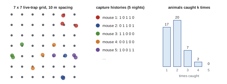
print("frequency of capture counts (1..5 times):", f.tolist())individuals caught at least once: 46 of 54 nights 1-2: n1 = 21, n2 = 13, m2 = 5; Chapman N = 50 (95% CI 26 to 75) Schnabel N over 5 nights = 54 (true 54) frequency of capture counts (1..5 times): [17, 20, 7, 2, 0]
The frequencies of capture counts, how many animals were caught once, twice and so on, are what heterogeneity models use: an excess of animals caught only once suggests that some individuals are much harder to catch. Chao's heterogeneity estimator for this situation is closely related to the Chao1 species richness estimator from BIOL-367, which uses the numbers of species seen once and twice in the same way.
Open populations
Over longer periods, populations are open: animals are born, die and move. The Jolly–Seber model estimates abundance, survival and recruitment for each interval from repeated sampling of marked and unmarked animals. The Cormack–Jolly–Seber model uses only marked animals to estimate apparent survival, survival confounded with permanent emigration, and is the workhorse of avian and mammal demography; band recovery and resighting data from long-term banding programs feed it. Pollock's robust design combines the two time scales: primary periods months apart, each containing several closely spaced secondary occasions, so closed models estimate abundance within periods and open models estimate survival and movement between them. The deer mouse study uses a robust design with five-night sessions in June, July and August.
Removal sampling
If animals are removed, or marked so that they are not counted again, the catch should decline from one pass to the next because fewer remain. Electrofishing in a stream section blocked by nets, repeated sweeps for amphibians in a small pond and successive trap nights where captured animals are not released all produce removal data. With two passes and constant capture probability, \(\hat{N} = C_1^2/(C_1 - C_2)\) and \(\hat{p} = (C_1 - C_2)/C_1\). The estimate is unstable if the second catch is close to the first, which happens when capture probability is low. Zippin's maximum likelihood method extends this to three or more passes.
# Removal sampling of tiger salamander larvae in a small wetland (synthetic): two-pass and three-pass estimates.
import numpy as np
rng = np.random.default_rng(8)
N_true, p = 140, 0.45
remaining = N_true; catches = []
for _ in range(3):
    c = rng.binomial(remaining, p); catches.append(c); remaining -= c
C1, C2, C3 = catches
print("catches per pass:", catches)
print(f"two-pass: N = {C1**2 / (C1 - C2):.0f}, p = {(C1 - C2) / C1:.2f}")
T = sum(catches); k = len(catches)
from math import lgamma, log
def loglik(N, q):
    ll = lgamma(N + 1) - lgamma(N - T + 1)
    ll += sum(c * (log(q) + i * log(1 - q)) for i, c in enumerate(catches))
    return ll + (N - T) * k * log(1 - q)
best = max((loglik(N, q), N, q) for N in range(T, 400) for q in np.linspace(0.05, 0.95, 181))
print(f"three-pass maximum likelihood: N = {best[1]}, p = {best[2]:.2f} (true N = {N_true}, p = {p})")catches per pass: [60, 36, 24] two-pass: N = 150, p = 0.40 three-pass maximum likelihood: N = 156, p = 0.38 (true N = 140, p = 0.45)
In this simulated wetland both estimates overshoot the true 140 larvae because, by chance, the catch fell a little more slowly than expected, which the methods read as a lower capture probability. Removal estimates are sensitive to exactly this kind of sampling noise, and a fourth pass or a higher capture probability would narrow the gap.
Occupancy and repeated counts
Sometimes the question is not how many but where: which wetlands are occupied by boreal chorus frogs? Occupancy models, introduced by MacKenzie and colleagues in 2002 and covered briefly in BIOL-367, use repeated visits to each site to separate the probability that a site is occupied, \(\psi\), from the probability of detecting the species on a visit when it is there, \(p\). A site where frogs were heard on one of three visits is occupied; a site where they were never heard may be unoccupied or occupied and missed, and the pattern of detections across sites tells the model how likely the latter is.
Repeated counts at the same sites, rather than detections, support N-mixture models, developed by Royle in 2004. They assume that each site has a fixed local abundance \(N_i\) during the survey period, following a Poisson or negative binomial distribution, and that each count is a binomial sample of \(N_i\) with detection probability \(p\). Because the method needs no marking, it is popular for birds, amphibians and plants. Its estimates are sensitive to violations of closure, double counting and unmodelled heterogeneity in detection, so it works best with careful field protocols and is best treated with caution when counts are low.
Spatial capture–recapture and camera traps
Classical mark–recapture estimates abundance but not the area it applies to, because animals living near the edge of a trapping grid use areas outside it. Ad hoc fixes, such as adding a boundary strip of half the mean distance between recaptures, are crude. Spatial capture–recapture models, developed by Efford, Borchers, Royle and others since about 2004, treat each animal as having an unobserved activity centre and model capture probability as declining with distance between the trap and that centre. They estimate density directly and are now standard for carnivores such as wolverines, grizzly bears and martens, using live traps, hair snares that collect DNA or camera traps for individually recognizable species such as lynx and bobcats.
Camera traps have transformed mammal surveys. For species without individual markings, such as white-tailed deer or coyotes, methods such as random encounter models, time-to-event and space-to-event models, and camera trap distance sampling estimate density from detection rates and camera fields of view. Canadian national parks and many state agencies now run camera networks, and machine learning tools sort millions of images, though human checking remains important for rare species and errors.
Environmental DNA and detection
Environmental DNA, eDNA, refers to genetic material shed by organisms into water, soil or air. A litre of wetland water, filtered and analysed by quantitative PCR for a species-specific marker or by metabarcoding for many species at once, can reveal the presence of frogs, salamanders, fish or invasive mussels without seeing them. eDNA has its own detection problem: DNA may be absent from a particular sample even when the species is present, a PCR replicate may fail to amplify DNA that is in the sample, and contamination can produce false positives. Multi-scale occupancy models handle these levels: site occupancy, presence in a water sample and detection in a PCR replicate.
# How many water samples and qPCR replicates are needed to detect a species with eDNA?
theta = 0.55    # probability that a 1 L sample from an occupied wetland contains the target DNA
p_pcr = 0.70    # probability that one qPCR replicate amplifies DNA present in a sample
for samples in (1, 2, 3, 4):
    row = []
    for reps in (1, 3, 6):
        per_sample = theta * (1 - (1 - p_pcr) ** reps)
        row.append(1 - (1 - per_sample) ** samples)
    print(f"{samples} samples: detection with 1, 3, 6 replicates = " + ", ".join(f"{r:.2f}" for r in row))
print("negative controls at every step guard against false positives from contamination")1 samples: detection with 1, 3, 6 replicates = 0.39, 0.54, 0.55 2 samples: detection with 1, 3, 6 replicates = 0.62, 0.78, 0.80 3 samples: detection with 1, 3, 6 replicates = 0.77, 0.90, 0.91 4 samples: detection with 1, 3, 6 replicates = 0.86, 0.95, 0.96 negative controls at every step guard against false positives from contamination
The calculation shows a common finding: once each sample has three or more PCR replicates, adding replicates helps little, because the limiting factor is whether a sample captures DNA at all, and adding water samples is more effective. Field and laboratory negative controls, blanks of clean water handled exactly like samples, are essential to detect contamination.
| Method | Field data | Estimates | Main assumptions or limits |
|---|---|---|---|
| Lincoln–Petersen or Chapman | Two capture sessions of marked animals | Abundance | Closure, no mark loss, equal catchability |
| Closed models (M0, Mt, Mb, Mh) | Capture histories over several occasions | Abundance and capture probability | Closure; models for variation in capture |
| Cormack–Jolly–Seber | Recaptures or resightings of marked animals over years | Apparent survival and recapture probability | Emigration confounded with death |
| Removal | Declining catches over passes | Abundance and capture probability | Closure, constant capture probability |
| Occupancy | Detection or non-detection on repeat visits | Occupancy and detection probability | Closure of occupancy during the season |
| N-mixture | Repeated counts at sites | Site abundance and detection probability | Closure, no double counts; sensitive to heterogeneity |
| Spatial capture–recapture | Captures with trap locations | Density, detection and movement scale | Activity centres fixed during survey |
Worked problem
A two-night estimate with assumptions
On night 1 the crew captures and ear-tags 31 deer mice. On night 2 it catches 28, of which 15 are tagged. Estimate abundance with Chapman's estimator and list two reasons the estimate could be biased.
Show solution
- Chapman N = (31 + 1)(28 + 1)/(15 + 1) - 1 = 32 x 29 / 16 - 1 = 58 - 1 = 57.
- Variance = 32 x 29 x 16 x 13 / (16^2 x 17) = 193,024 / 4,352 = about 44, so SE is about 6.7 and the 95 per cent interval is roughly 44 to 70.
- Trap-happiness after baited captures would raise recapture rates and bias N low.
- Mice living at the grid edge with home ranges partly outside it make the area to which N applies unclear; spatial capture–recapture addresses this.
Answer: About 57 mice (roughly 44 to 70), with possible bias from trap response and edge effects.
Common mistakes
MistakeRunning a mark–recapture study over a whole season and treating it as closed.
InsteadUse short sessions for closed models, or open models such as Jolly–Seber or the robust design.
MistakeAssuming all animals are equally catchable.
InsteadFit models with behavioural responses and heterogeneity, and compare them.
MistakeConverting a grid abundance to density using only the grid area.
InsteadAccount for animals using areas beyond the grid, ideally with spatial capture–recapture.
MistakeTreating eDNA non-detection as proof of absence.
InsteadEstimate detection at the sample and PCR levels and replicate accordingly.
MistakeUsing N-mixture models on low counts with heterogeneous detection without checks.
InsteadUse careful protocols, check assumptions and interpret cautiously.
Summary and key terms
- Mark–recapture estimates abundance from the fraction of marked animals in later samples; Chapman's estimator reduces small-sample bias.
- Closure, intact marks and equal catchability are key assumptions; multi-occasion models test and relax them.
- Open-population models estimate survival and recruitment; the robust design combines open and closed periods.
- Removal sampling estimates abundance from declining catches.
- Occupancy and N-mixture models use repeated visits to separate presence or abundance from detection.
- Spatial capture–recapture estimates density directly; camera traps and eDNA extend detection, each with their own detection models.
- Lincoln–Petersen estimator
- Abundance estimate n1 n2 / m2 from two capture sessions.
- closed population
- A population with no births, deaths or movement during the study period.
- trap-happy
- Describes animals more likely to be recaptured after first capture.
- capture history
- A record of whether an individual was caught on each occasion.
- apparent survival
- Survival estimated from recaptures, confounded with permanent emigration.
- robust design
- Sampling with closely spaced secondary occasions nested within widely spaced primary periods.
- removal sampling
- Estimating abundance from declining catches as animals are removed.
- N-mixture model
- A model estimating site abundance and detection probability from repeated counts.
- spatial capture–recapture
- Models that estimate density using trap locations and animals' activity centres.
- environmental DNA
- Genetic material shed into the environment and used to detect species.
Practice problems
Work each problem on paper first, then reveal the answer to check.
n1 = 40, n2 = 50, m2 = 20. Compute the Lincoln–Petersen estimate.
Show answer
40 x 50 / 20 = 100.
Compute Chapman's estimate for the same data.
Show answer
41 x 51 / 21 - 1 = 98.6, about 99.
Which model letter describes a behavioural response to capture?
Show answer
Mb.
Two-pass removal catches are 60 and 30. Estimate N and p.
Show answer
N = 3,600/30 = 120; p = 30/60 = 0.5.
What does a Cormack–Jolly–Seber model estimate?
Show answer
Apparent survival and recapture probability.
Why does a removal estimate become unstable when C2 is close to C1?
Show answer
The denominator C1 - C2 is small, so small changes give large swings; capture probability is low.
In eDNA surveys, what do field blanks detect?
Show answer
Contamination that could cause false positives.
What problem of classical grids does spatial capture–recapture solve?
Show answer
It estimates density directly by modelling activity centres, so the effective area is not assumed.
Lesson quiz · 5 questions
Score 60% or more to complete this lesson.
Create a free account to save your progress, take quizzes and earn a certificate.