
BIOL-430 · Lesson 12 of 12 · 26 min
Capstone: long-term monitoring, open data and a field study proposal
Some of the most important things ecologists have learned came from studies that ran for decades: the links between snowshoe hares and lynx, the effects of acid rain on lakes, the advance of spring, the decline of grassland birds. Short studies cannot see slow change, rare events or lagged responses. This capstone lesson pulls the course together around three themes: long-term monitoring and what makes it worth the effort; open, well-documented data that others can reuse; and writing a field study proposal, illustrated by the team's plan to turn the four-year grazing study into a long-term monitoring program at the field station. Along the way it completes the BACI analysis begun in lesson 2.
Why long-term studies matter
Ecological processes run on many time scales. Wetland plant communities in the prairie pothole region cycle with wet and dry periods lasting years to decades, so a three-year study could easily see only a drought or only a deluge. Many species are long-lived, so populations respond to change with lags; some effects, such as soil carbon change under altered grazing, take a decade or more to measure. Rare events, such as a once-in-50-years flood, a disease outbreak or an extreme heat wave, may drive more change than average conditions, and only long records capture them. Long series also provide the baselines without which change cannot be recognized at all, the problem known as shifting baselines.
Several programs show what long-term work achieves. The United States Long Term Ecological Research (LTER) Network, funded by the National Science Foundation since 1980, now comprises 26 sites, from the Arctic tundra to coral reefs to the Konza Prairie tallgrass site in Kansas and the Cedar Creek Ecosystem Science Reserve in Minnesota, where long-running biodiversity experiments have shown how plant diversity affects productivity and stability. The National Ecological Observatory Network (NEON), also NSF-funded, collects standardized data at about 80 sites across the country. In Canada, the IISD Experimental Lakes Area in northwestern Ontario has run whole-lake experiments on 58 small lakes since 1968, showing how phosphorus, acid rain, mercury and other stressors affect freshwater ecosystems; the Kluane Boreal Forest Ecosystem Project in Yukon, from 1986 to 1996, manipulated food and predators at large scale to explain the snowshoe hare cycle; and the Churchill Northern Studies Centre in Manitoba supports long-term subarctic research. Lesson 7's Breeding Bird Survey (since 1966) and Christmas Bird Count (since 1900) are long-term programs powered by volunteers.
| Program | Where | Since | Known for |
|---|---|---|---|
| Christmas Bird Count | Across the Americas | 1900 | Winter bird distributions and range shifts |
| North American Breeding Bird Survey | Canada and United States | 1966 | Breeding bird population trends, including grassland bird declines |
| IISD Experimental Lakes Area | Northwestern Ontario | 1968 | Whole-lake experiments on nutrients, acidification, mercury |
| LTER Network | United States, 26 sites | 1980 | Long-term ecosystem research across biomes |
| Kluane Boreal Forest Ecosystem Project | Yukon | 1986 to 1996 | Large-scale experiments on the snowshoe hare cycle |
| NEON | United States, about 80 sites | full operation from 2019 | Standardized continental ecological data |
Detecting change: power for monitoring
Monitoring programs need their own power analysis, framed in terms of trends: how many years, sites and visits are needed to detect a decline of a given rate? The answer depends on the size of the trend, the year-to-year variation in the index, the number of sites and whether the same sites are revisited, which removes persistent differences among sites in the same way a BACI design does. Gerrodette's work in the 1980s and many later simulation studies show that detecting a 2 per cent annual decline, which halves a population in about 35 years, often takes 10 to 20 years of data. That sobering result argues for designing monitoring programs to last, choosing indices with low variance and revisiting the same sites.
# Years of monitoring needed to detect a 2% annual decline in sparrow counts (synthetic, revisited sites).
import numpy as np
rng = np.random.default_rng(2026)
def power(years, sites=30, trend=-0.02, year_sd=0.15, site_sd=0.5, sims=600):
    hits = 0
    t = np.arange(years)
    for _ in range(sims):
        yr = rng.normal(0, year_sd, years)
        site = rng.normal(0, site_sd, sites)
        lam = np.exp(np.log(6) + site[:, None] + (trend * t + yr)[None, :])
        y = rng.poisson(lam)
        idx = np.log(y.mean(0) + 0.5)                     # annual index across revisited sites
        X = np.column_stack([np.ones(years), t])
        b, res = np.linalg.lstsq(X, idx, rcond=None)[:2]
        s2 = res[0] / (years - 2)
        se = np.sqrt(s2 * np.linalg.inv(X.T @ X)[1, 1])
        hits += b[1] / se < -2.0                           # one-sided test, roughly alpha = 0.05
    return hits / sims
for years in (5, 10, 15, 20):
    print(f"{years:2d} years, 30 sites: power to detect a 2%/yr decline = {power(years):.2f}")
print(f"10 years with half the year-to-year noise: power = {power(10, year_sd=0.075):.2f}")5 years, 30 sites: power to detect a 2%/yr decline = 0.12 10 years, 30 sites: power to detect a 2%/yr decline = 0.22 15 years, 30 sites: power to detect a 2%/yr decline = 0.48 20 years, 30 sites: power to detect a 2%/yr decline = 0.86 10 years with half the year-to-year noise: power = 0.41
The simulation shows that five years of monitoring has little chance of detecting a moderate decline, and that reducing year-to-year noise, for example by standardizing survey timing and conditions or by modelling detection, helps as much as many more sites. Because shared year effects affect all sites together, adding sites cannot average them away; only more years can.
Adaptive management
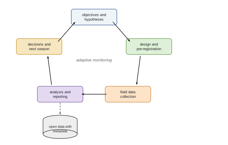
Monitoring is most valuable when it feeds decisions. Adaptive management, developed by Holling, Walters and colleagues in the 1970s and 1980s, treats management actions as experiments: state objectives and competing hypotheses about how the system will respond, choose actions, monitor the results and update both understanding and actions. The North American waterfowl harvest is a long-running example: since 1995 the United States Fish and Wildlife Service has set duck hunting regulations using adaptive harvest management, which weights competing population models by how well they predicted past outcomes, informed by the breeding population surveys described in lesson 5. The grazing study can work the same way: the ranch's objectives, such as forage production and nesting cover, are explicit; the competing hypotheses about how fencing and rotation affect them are written down; and annual monitoring informs whether to extend fencing to more wetlands.
Completing the grazing BACI analysis
After four seasons, two before fencing and two after, the team analyses edge vegetation height at the twelve fenced and twelve control wetlands. Following the plan registered before data collection, the response for each wetland is the change in mean height from the before period to the after period, and the treatment effect is the difference in mean change between fenced and control wetlands, tested by permutation of treatment labels within pasture pairs, which respects the blocked design of lesson 2.
# Final BACI analysis: edge vegetation height at 12 fenced and 12 control wetlands, 2 years before and 2 after.
import numpy as np
rng = np.random.default_rng(430)
pairs = 12
site = rng.normal(0, 9, (pairs, 2)) + np.array([6.0, 0.0])   # persistent differences; the ranch fenced wetter sites
year = np.array([0.0, -6.0, 3.0, 5.0])                   # shared year effects: year 2 was a drought
y = 52 + site[:, :, None] + year[None, None, :] + rng.normal(0, 6, (pairs, 2, 4))
y[:, 0, 2:] += 11.0                                      # column 0 of each pair was fenced after year 2
change = y[:, :, 2:].mean(2) - y[:, :, :2].mean(2)       # after minus before, per wetland
diff = change[:, 0] - change[:, 1]                       # fenced minus control within each pair
obs = diff.mean()
flips = rng.choice([-1, 1], (20000, pairs))
null = (flips * diff).mean(1)
p = (1 + np.sum(np.abs(null) >= abs(obs))) / (1 + len(null))
se = diff.std(ddof=1) / np.sqrt(pairs)
print(f"mean change: fenced {change[:, 0].mean():+.1f} cm, control {change[:, 1].mean():+.1f} cm")
print(f"BACI effect = {obs:.1f} cm (95% CI {obs - 2.2 * se:.1f} to {obs + 2.2 * se:.1f}), permutation p = {p:.4f}")
print(f"naive after-only comparison: {y[:, 0, 2:].mean() - y[:, 1, 2:].mean():.1f} cm")mean change: fenced +18.5 cm, control +4.5 cm BACI effect = 14.0 cm (95% CI 8.9 to 19.1), permutation p = 0.0007 naive after-only comparison: 19.7 cm
The result supports the hypothesis that excluding cattle increases edge vegetation height. The point estimate, about 14 centimetres, exceeds the 10 centimetres the team identified in lesson 1 as the smallest effect that matters for nest concealment, although the lower end of the confidence interval falls just below that threshold, so the evidence that the effect is ecologically important, as opposed to merely real, is strong but not conclusive. The drought in year 2 lowered heights everywhere, which a before–after comparison at fenced wetlands alone would have mistaken for part of the effect, and the after-only comparison is inflated because the ranch had fenced wetlands that were already taller, a pre-existing difference the BACI design removes. Because fencing was not randomized, the team also checks that fenced and control wetlands followed similar trends in the two pre-treatment years, the only available test of parallel trends, and reports it alongside the result.
Open data and reproducibility
Data that sit on a laptop help no one and are eventually lost. Funders and journals in both countries increasingly require data to be deposited in public repositories, and the FAIR principles, published in 2016, ask that data be findable, accessible, interoperable and reusable: with persistent identifiers such as DOIs, rich metadata, open formats and clear licences. Ecological data repositories include Dryad, the Environmental Data Initiative (which archives LTER data), DataONE, which links many repositories, the Global Biodiversity Information Facility (GBIF) for species occurrences and Movebank for animal tracking data. Reproducibility also means sharing code: analysis scripts under version control, with a record of software versions, allow others, including reviewers, to rerun the analysis.
In Canada, the Tri-Agency Research Data Management Policy requires institutions to have data management strategies and asks researchers to submit data management plans with certain funding applications and to deposit data supporting publications. Canadian repositories include Borealis, the Canadian Dataverse Repository, the Federated Research Data Repository run by the Digital Research Alliance of Canada, and the Polar Data Catalogue for northern research. Data from First Nations partners are shared only as the data agreement allows, following OCAP.
Open data and ethics can conflict. Locations of species at risk, cultural sites and private land details may need to be generalized, embargoed or restricted, and Indigenous data governance means that some data belong to communities and are shared on their terms. Open by default does not mean open without judgment; it means that restrictions are deliberate, documented and justified.
Writing a field study proposal
A field study proposal persuades a funder, a committee or a partner that the work is worth doing and will succeed. Most share a structure: a summary; background that establishes the problem and the gap in knowledge; objectives and hypotheses with explicit predictions; study area; design, including sampling units, treatments, controls, replication and the power analysis behind them; field methods and data quality procedures; analysis plan; permits, ethics and community engagement; safety and biosecurity; data management and sharing; timeline; budget; and expected outcomes and their use. Reviewers look for a clear question, a design that can answer it, realistic logistics and evidence that the team has anticipated what could go wrong.
| Proposal section | What the grazing monitoring proposal says (summary) |
|---|---|
| Question | How do wetland-margin fencing and rotational grazing affect edge vegetation, grassland birds, small mammals and amphibians over ten years? |
| Hypotheses and predictions | Fencing increases residual cover; bird density and amphibian occupancy rise with cover; effects vary with wet and dry years |
| Design | Expand the BACI to 24 fenced and 24 control wetlands in pairs within pastures; revisit annually |
| Power | Simulation: 24 pairs detect a 5 cm height effect with power about 0.8; 15 to 20 years are needed for good power to detect a 2 per cent annual bird trend |
| Methods | Daubenmire quadrats, Robel pole, point-transect distance sampling, deer mouse robust-design trapping, frog call and eDNA surveys, loggers, Sentinel-2 NDVI |
| Analysis | GLMMs with wetland and year random effects; distance and occupancy models; PERMANOVA for plant composition; pre-registered |
| Permits and partners | Provincial or state permits, animal care, banding permits, ranch agreement, Indigenous data agreement |
| Safety and biosecurity | Field safety plan with check-ins; tick and hantavirus protocols; clean, drain, dry |
| Data | Tidy database with EML metadata; annual deposit to a public repository with sensitive locations generalized |
| Use | Annual report to the ranch and partners for adaptive decisions on extending fencing |
Pre-registration in practice
The team pre-registers the monitoring plan on a public registry before the next field season, stating the primary response variables, the model, the expected direction of effects, how missing data and outliers will be handled and which analyses are exploratory. Pre-registration is not a straitjacket: field studies change, a flood may wipe out a season or a new question may arise, and deviations are acceptable if they are reported openly. Registered reports, in which journals review and accept the plan before data are collected, go further, removing the pressure to obtain significant results.
Field ecology in a changing world
The skills in this course are increasingly in demand. Climate change is shifting phenology and ranges, as long records of flowering dates, bird migration and tick-borne disease show; habitat conversion continues to remove prairie wetlands and grasslands; and environmental assessment, species-at-risk recovery, agricultural sustainability programs and carbon markets all depend on reliable field data. The future of the field combines old and new: careful observation and natural history, which no sensor replaces, with drones, autonomous recorders, eDNA, satellite imagery and statistical models that make the most of every observation. BIOL-440 and BIOL-460 apply these methods to boreal and northern ecosystems and to lakes and rivers, and the honours research project, BIOL-499, is the place to carry out a study of your own design.
Worked problem
Checking the parallel-trends assumption
In the two pre-treatment years, fenced wetlands averaged 50.1 and 44.0 cm and controls 47.8 and 41.5 cm. After fencing, fenced wetlands averaged 66.0 and 68.2 cm and controls 51.0 and 52.9 cm. Check pre-treatment trends and compute the BACI effect.
Show solution
- Pre-treatment change: fenced 44.0 - 50.1 = -6.1 cm; control 41.5 - 47.8 = -6.3 cm. The trends are nearly parallel, which supports the assumption.
- Before means: fenced 47.05, control 44.65. After means: fenced 67.1, control 51.95.
- Changes: fenced +20.05, control +7.30.
- BACI effect = 20.05 - 7.30 = 12.75 cm.
Answer: Pre-treatment trends are parallel (-6.1 vs -6.3 cm), and the BACI estimate is about 12.8 cm.
Common mistakes
MistakeStarting a monitoring program without a power analysis for trends.
InsteadSimulate how many years, sites and visits are needed to detect the trends that matter.
MistakeChanging methods partway through a long-term program without calibration.
InsteadRun old and new methods side by side before switching, and document the change.
MistakeArchiving data without metadata.
InsteadDeposit data with EML or equivalent metadata, code and a clear licence.
MistakePublishing exact locations of sensitive species and cultural sites.
InsteadGeneralize or restrict sensitive data deliberately and document the reasons.
MistakeTreating monitoring as an end in itself.
InsteadLink monitoring to objectives, hypotheses and decisions through adaptive management.
Summary and key terms
- Long-term studies capture slow change, lags, rare events and baselines that short studies miss.
- Monitoring power depends mostly on year-to-year variation and the number of years; detecting moderate trends often needs a decade or more.
- Adaptive management links monitoring to decisions by treating actions as experiments.
- The grazing BACI analysis estimated a fencing effect on edge height above the 10 cm threshold that matters for nesting cover, after checking pre-treatment trends.
- FAIR data, repositories, metadata and shared code make field research reusable and reproducible, with deliberate limits for sensitive and Indigenous data.
- Strong proposals state a clear question, a powered design, realistic logistics, ethics, safety and data plans.
- long-term ecological research
- Sustained study of ecological systems over decades to capture slow and rare processes.
- shifting baselines
- The loss of awareness of past conditions when each generation accepts the current state as normal.
- monitoring power
- The probability that a monitoring program detects a trend of a given size.
- adaptive management
- Management that treats actions as experiments and updates decisions from monitoring results.
- permutation test
- A test comparing an observed statistic with its distribution under random relabelling of treatments.
- FAIR principles
- Guidelines that data be findable, accessible, interoperable and reusable.
- data repository
- A service that stores, preserves and provides access to research data with persistent identifiers.
- registered report
- A publication format in which the study plan is peer reviewed and accepted before data collection.
- NEON
- The National Ecological Observatory Network, collecting standardized ecological data across the United States.
- LTER Network
- The US Long Term Ecological Research Network of NSF-funded research sites.
Practice problems
Work each problem on paper first, then reveal the answer to check.
A population declines 2 per cent a year. Roughly how long until it halves?
Show answer
About 35 years (ln 2 / 0.02).
Why can more sites not overcome shared year-to-year variation in a trend analysis?
Show answer
Year effects affect all sites together, so only more years average them out.
Name two Canadian and two United States long-term ecological programs.
Show answer
For example IISD Experimental Lakes Area and the Kluane project; the LTER Network and NEON.
What does adaptive harvest management do with competing population models?
Show answer
Weights them by how well they predicted past outcomes and uses them to set regulations.
What does the F in FAIR stand for, and how is it achieved?
Show answer
Findable: persistent identifiers such as DOIs and rich metadata.
In the final BACI analysis, why permute within pasture pairs?
Show answer
To respect the blocked design, so the null distribution matches how treatments were assigned.
List four sections every field proposal should contain.
Show answer
For example question and hypotheses, design and power, methods, and data management.
Why might some data from the study not be fully public?
Show answer
Sensitive species locations, private land details or Indigenous data governed by partner agreements.
Lesson quiz · 5 questions
Score 60% or more to complete this lesson.
Create a free account to save your progress, take quizzes and earn a certificate.