
BIOL-430 · Lesson 11 of 12 · 28 min
Analysing field data: GLMs, mixed models and ordination
By the end of a field season the team has thousands of records: quadrat cover estimates, Robel readings, bird detections with distances, mouse capture histories, deer locations, water chemistry, logger files and photographs. Turning them into conclusions requires three things: clean, well-documented data; statistical models that match the structure of the data, which in ecology means counts, proportions, presence and absence, nested sampling and repeated measures; and multivariate tools for whole communities. This lesson covers data management and quality control, generalized linear models for counts and binary data, mixed models for nested designs, ordination of community data and model selection. STAT-151 covered linear regression and analysis of variance; here we extend them to the kinds of data field ecologists actually collect.
From field sheet to tidy data
Data management starts in the field. Paper data sheets or tablet forms should record who, where, when, how and what for every observation, with controlled vocabularies such as four-letter species codes, validated ranges for numbers and required fields so that blanks mean something. Tablet forms with drop-down lists and range checks prevent many errors at entry; paper sheets need double entry or careful proofreading. Photographs of paper sheets at the end of each day protect against loss. Raw data files should never be edited by hand once checked: corrections are made by scripts that read the raw file and write a cleaned version, so every change is documented and reproducible.
Tidy data, a term popularized by Hadley Wickham, follow three rules: each variable is a column, each observation is a row and each type of observational unit is a table. A survey might have a table of sites, with coordinates and treatment; a table of visits, with date, observer and weather; and a table of observations, one row per species per quadrat per visit, linked by identifiers. This structure makes analysis straightforward and avoids the wide spreadsheets with one column per species per date that field data so often end up in.
# Quality control of a tidy quadrat table before analysis (synthetic records with planted errors).
import pandas as pd
rows = [
    ('W03', '2026-07-08', 'LT', 'CAAT', 35), ('W03', '2026-07-08', 'LT', 'TYLA', 20),
    ('W03', '2026-07-08', 'LT', 'HOJU', 5),  ('W07', '2026-07-08', 'PN', 'CAAT', 140),
    ('W07', '2026-07-08', 'PN', 'CXAT', 15), ('W11', '2026-07-09', 'PN', 'TYLA', 30),
    ('W11', '2026-07-09', 'PN', 'TYLA', 30), ('W15', '2026-07-31', 'SW', 'SCFE', 25),
    ('W19', '2026-07-10', None, 'HOJU', 10),
]
df = pd.DataFrame(rows, columns=['wetland', 'date', 'observer', 'species', 'cover'])
codes = {'CAAT', 'TYLA', 'HOJU', 'SCFE', 'POPR', 'JUBA'}
season = ('2026-07-01', '2026-07-20')
checks = {
    'cover outside 0-100': df[(df.cover < 0) | (df.cover > 100)],
    'unknown species code': df[~df.species.isin(codes)],
    'duplicate record': df[df.duplicated(keep='first')],
    'date outside sampling window': df[(df.date < season[0]) | (df.date > season[1])],
    'missing observer': df[df.observer.isna()],
}
for name, bad in checks.items():
    for _, r in bad.iterrows():
        print(f"{name:28s} {r.wetland} {r.date} {r.species} cover={r.cover}")
print(f"{sum(len(b) for b in checks.values())} problems flagged in {len(df)} records; fix in the cleaning script, never in the raw file")cover outside 0-100 W07 2026-07-08 CAAT cover=140 unknown species code W07 2026-07-08 CXAT cover=15 duplicate record W11 2026-07-09 TYLA cover=30 date outside sampling window W15 2026-07-31 SCFE cover=25 missing observer W19 2026-07-10 HOJU cover=10 5 problems flagged in 9 records; fix in the cleaning script, never in the raw file
Metadata, the documentation that makes data understandable to someone else, or to yourself in five years, describes the study, methods, units, codes, coordinate systems and known problems. Ecological Metadata Language (EML) is a standard used by the LTER network and data repositories; even a well-written plain-text file listing every variable, its units and its allowed values is far better than nothing. Lesson 12 discusses archiving and sharing.
Generalized linear models
Ordinary linear regression assumes that the response is continuous, that residuals are normally distributed with constant variance and that effects are additive. Counts of birds or plants, proportions of seedlings surviving and presence or absence of frogs violate all three. Generalized linear models (GLMs) handle them with two components: a probability distribution for the response, such as Poisson or negative binomial for counts and binomial for successes out of trials or presence and absence; and a link function connecting the mean of the response to a linear predictor. For counts the usual link is the log, \(\log \mu = \beta_0 + \beta_1 x_1 + \dots\), so effects multiply the mean: a coefficient of 0.2 means each unit of \(x\) multiplies the expected count by \(e^{0.2} = 1.22\). For binary data the logit link, \(\log[p/(1-p)]\), gives coefficients interpreted as log odds ratios.
When counts come from units of different size or effort, such as transects of different lengths or trap grids open for different numbers of nights, an offset, the log of effort, enters the linear predictor with a fixed coefficient of 1, so that the model describes counts per unit effort.
Overdispersion
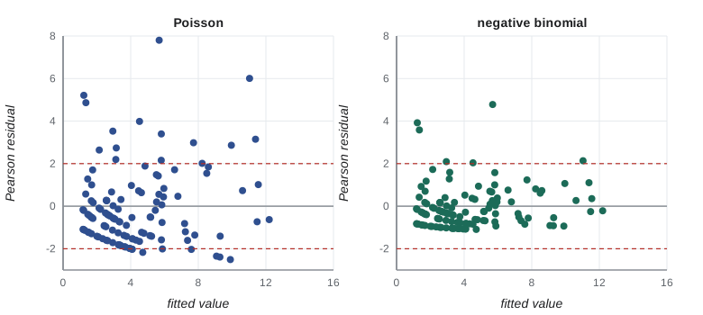
The Poisson distribution assumes the variance equals the mean. Ecological counts are almost always more variable, because of unmeasured habitat differences, clumping and individual heterogeneity, as lesson 5 showed for quadrat counts. Fitting a Poisson GLM to overdispersed data gives standard errors that are too small and p-values that are too optimistic. A simple diagnostic is the ratio of the Pearson chi-squared statistic to residual degrees of freedom: values well above 1 indicate overdispersion. Remedies include the negative binomial GLM, which adds a parameter for extra variation; quasi-Poisson models, which scale standard errors by the dispersion; and random effects for the units that cause the extra variation. When there are more zeros than either distribution predicts, zero-inflated or hurdle models separate the processes that produce zeros, such as unsuitable sites versus suitable but unoccupied ones.
# Poisson vs negative binomial GLM: savannah sparrow counts per point vs visual obstruction (synthetic).
import numpy as np
from scipy import optimize, special
rng = np.random.default_rng(1110)
n = 120
vo = rng.uniform(0.5, 6, n)                           # Robel visual obstruction (dm)
mins = rng.choice([5, 10], n)                         # count duration (min): an offset
mu = np.exp(-1.6 + 0.30 * vo) * mins
y = rng.negative_binomial(2.0, 2.0 / (2.0 + mu))      # overdispersed counts
X = np.column_stack([np.ones(n), vo]); off = np.log(mins)
def pois_nll(b):
    eta = X @ b + off
    return -np.sum(y * eta - np.exp(eta) - special.gammaln(y + 1))
def nb_nll(p):
    b, k = p[:2], np.exp(p[2]); m = np.exp(X @ b + off)
    return -np.sum(special.gammaln(y + k) - special.gammaln(k) - special.gammaln(y + 1)
                   + k * np.log(k / (k + m)) + y * np.log(m / (k + m)))
fp = optimize.minimize(pois_nll, np.zeros(2), method='BFGS')
fn = optimize.minimize(nb_nll, np.r_[fp.x, 0.0], method='BFGS')
m = np.exp(X @ fp.x + off)
disp = np.sum((y - m) ** 2 / m) / (n - 2)
for name, f, k in [('Poisson', fp, 2), ('negative binomial', fn, 3)]:
    se = np.sqrt(np.diag(f.hess_inv))[1]
    print(f"{name:18s} slope {f.x[1]:.3f} (SE {se:.3f}), AIC {2 * f.fun + 2 * k:.1f}")
print(f"Poisson dispersion ratio = {disp:.2f}; NB size parameter k = {np.exp(fn.x[2]):.2f}")
print(f"each extra dm of visual obstruction multiplies expected count by {np.exp(fn.x[1]):.2f}")Poisson slope 0.398 (SE 0.031), AIC 716.0 negative binomial slope 0.352 (SE 0.055), AIC 576.1 Poisson dispersion ratio = 3.83; NB size parameter k = 1.58 each extra dm of visual obstruction multiplies expected count by 1.42
Both models estimate a similar slope, but the Poisson model's standard error is too small, because it ignores the extra variation that the dispersion ratio reveals, and its AIC is much worse. In practice, the negative binomial is the default starting point for ecological counts, and the dispersion check should be routine.
Mixed models for nested designs
Field data are almost always grouped: quadrats within wetlands, wetlands within pastures, repeated visits to the same points, several years at the same sites. Observations within a group share unmeasured influences and so are correlated, the problem of pseudoreplication from lesson 2. Mixed models, also called hierarchical or multilevel models, handle this by including random effects, such as a random intercept for each wetland, that represent the deviation of each group from the overall mean, drawn from a normal distribution with a variance estimated from the data. Fixed effects, such as treatment, period and their interaction in a BACI design, are estimated against the appropriate level of variation. Generalized linear mixed models (GLMMs) combine random effects with Poisson, negative binomial or binomial responses. In R, the lme4 and glmmTMB packages are standard; in Python, statsmodels and Bayesian tools such as PyMC.
Random effects are appropriate for grouping factors whose levels are a sample from a larger set, such as wetlands, observers or years, when you want to generalize beyond the particular levels and when there are enough levels, ideally five or more, to estimate a variance. Factors whose specific levels are of interest, such as treatment, are fixed. A random effect also partially pools estimates: wetlands with few observations are pulled toward the overall mean, which improves estimates for poorly sampled groups.
# Why grouping matters: a slope estimated from quadrats nested in wetlands (synthetic).
import numpy as np
rng = np.random.default_rng(77)
J, q = 16, 12                                           # 16 wetlands, 12 quadrats each
moist = np.repeat(rng.uniform(15, 45, J), q)             # wetland-level predictor (soil moisture %)
u = np.repeat(rng.normal(0, 10, J), q)                    # wetland random effect, SD 10 cm
y = 30 + 0.9 * moist + u + rng.normal(0, 6, J * q)        # edge height (cm)
X = np.column_stack([np.ones(J * q), moist])
b = np.linalg.lstsq(X, y, rcond=None)[0]
res = y - X @ b
se_naive = np.sqrt(res @ res / (J * q - 2) * np.linalg.inv(X.T @ X)[1, 1])
ym = y.reshape(J, q).mean(1); xm = moist.reshape(J, q).mean(1)
Xm = np.column_stack([np.ones(J), xm]); bm = np.linalg.lstsq(Xm, ym, rcond=None)[0]
rm = ym - Xm @ bm
se_group = np.sqrt(rm @ rm / (J - 2) * np.linalg.inv(Xm.T @ Xm)[1, 1])
within = np.mean([np.var(y.reshape(J, q)[j], ddof=1) for j in range(J)])
between = np.var(ym, ddof=1) - within / q
print(f"slope ignoring wetlands: {b[1]:.2f} (SE {se_naive:.3f}, treats {J * q} quadrats as independent)")
print(f"slope from wetland means: {bm[1]:.2f} (SE {se_group:.3f}, {J} independent units)")
print(f"variance components: between wetlands {between:.0f}, within wetlands {within:.0f}; intraclass correlation {between / (between + within):.2f}")slope ignoring wetlands: 1.21 (SE 0.097, treats 192 quadrats as independent) slope from wetland means: 1.21 (SE 0.306, 16 independent units) variance components: between wetlands 192, within wetlands 33; intraclass correlation 0.85
The intraclass correlation, the share of variance that lies between groups, tells you how much the grouping matters. When it is high, as here, adding quadrats within wetlands adds little information about wetland-level effects, and the effective sample size is closer to the number of wetlands. A random-intercept mixed model would give essentially the wetland-means answer while using all the data and handling unequal numbers of quadrats.
Model selection
Ecologists usually have several plausible models. Burnham and Anderson popularized an approach based on information criteria: fit a small set of models, each representing a hypothesis chosen in advance, and rank them by Akaike's information criterion, \(AIC = -2\log L + 2k\), where \(L\) is the maximized likelihood and \(k\) the number of parameters. The model with the lowest AIC is best supported; differences, \(\Delta AIC\), of less than about 2 indicate substantial support for both models, and Akaike weights express the relative support for each model in the set. With small samples, the corrected AICc is preferred. AIC compares models fitted to the same data and says nothing about whether any of them fit well, so model checking with residual plots, dispersion tests and simulation remains essential. Fitting every possible combination of variables and choosing the best, so-called dredging, invites spurious results and is best reserved for exploration.
Ordination of communities
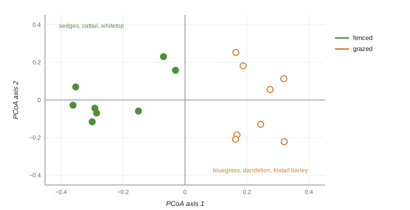
Community data, abundances or cover of many species at many sites, cannot be analysed one species at a time without losing the pattern. Ordination arranges sites in a low-dimensional space so that sites with similar composition are close together. Principal components analysis (PCA) works on correlations or covariances and suits short gradients with linear species responses. For typical community data, with many zeros and unimodal responses along long gradients, distance-based methods are better. Principal coordinates analysis (PCoA) and non-metric multidimensional scaling (NMDS) start from a dissimilarity matrix, most often Bray–Curtis, which for abundances \(x\) and \(y\) of species at two sites is \(BC = \sum |x_i - y_i| / \sum (x_i + y_i)\). NMDS seeks a configuration whose rank order of distances matches the rank order of dissimilarities, with stress measuring the mismatch.
Ordination is descriptive. To test whether composition differs between treatments, PERMANOVA (permutational multivariate analysis of variance) partitions variation in a dissimilarity matrix among factors and tests it by permutation, with permutations restricted to respect the design, for example within blocks. A significant PERMANOVA can reflect differences in spread rather than location, so a test of multivariate dispersion should accompany it. The vegan package in R implements these methods.
# Bray-Curtis dissimilarity and principal coordinates ordination of wetland-edge plant cover (synthetic).
import numpy as np
rng = np.random.default_rng(5150)
species = 12
fenced_profile = np.array([30, 18, 22, 6, 8, 2, 1, 0, 3, 5, 1, 0], float)
grazed_profile = np.array([14, 6, 3, 18, 20, 9, 7, 6, 10, 4, 2, 1], float)
sites = [rng.gamma(2, (fenced_profile + 0.5) / 2) for _ in range(8)] + [rng.gamma(2, (grazed_profile + 0.5) / 2) for _ in range(8)]
Y = np.array(sites); group = ['F'] * 8 + ['G'] * 8
D = np.array([[np.abs(a - b).sum() / (a + b).sum() for b in Y] for a in Y])
n = len(Y); Jc = np.eye(n) - 1 / n
B = -0.5 * Jc @ (D ** 2) @ Jc
vals, vecs = np.linalg.eigh(B); order = np.argsort(vals)[::-1]
vals, vecs = vals[order], vecs[:, order]
coords = vecs[:, :2] * np.sqrt(vals[:2])
pos = vals[vals > 0]
print(f"PCoA axes 1 and 2 explain {vals[0] / pos.sum():.0%} and {vals[1] / pos.sum():.0%} of positive variation")
for g in 'FG':
    c = coords[[i for i in range(n) if group[i] == g]]
    print(f"{'fenced' if g == 'F' else 'grazed'} centroid on axis 1: {c[:, 0].mean():+.3f}")
within = np.mean([D[i, j] for i in range(n) for j in range(i) if group[i] == group[j]])
between = np.mean([D[i, j] for i in range(n) for j in range(i) if group[i] != group[j]])
print(f"mean Bray-Curtis within groups {within:.2f}, between groups {between:.2f}")PCoA axes 1 and 2 explain 47% and 17% of positive variation fenced centroid on axis 1: -0.230 grazed centroid on axis 1: +0.230 mean Bray-Curtis within groups 0.39, between groups 0.60
| Data type | Typical model | Link | Watch for |
|---|---|---|---|
| Counts | Poisson or negative binomial GLM | log | Overdispersion, excess zeros, effort offsets |
| Presence or absence | Binomial GLM or occupancy model | logit | Imperfect detection |
| Successes out of trials | Binomial GLM | logit | Overdispersion among units |
| Continuous, positive | Gamma or log-normal model | log | Skewness, zeros |
| Grouped or repeated data | Mixed model with random effects | as above | Enough groups to estimate variance |
| Community composition | Ordination, PERMANOVA, joint species models | none or as above | Dissimilarity choice, dispersion differences |
Worked problem
Interpreting a GLM coefficient
A negative binomial GLM of sparrow counts gives a coefficient of 0.26 for visual obstruction (dm) and 0.41 for the fenced treatment after fencing. Interpret both on the count scale.
Show solution
- exp(0.26) = 1.30: each additional decimetre of visual obstruction multiplies expected counts by 1.30, a 30 per cent increase.
- exp(0.41) = 1.51: counts at fenced wetlands after fencing are about 51 per cent higher than predicted without the treatment effect, holding other terms constant.
- Report both with confidence intervals, and check that detection does not differ between treatments, as lesson 5 warned.
Answer: Counts rise about 30 per cent per decimetre of cover and are about 1.5 times higher at fenced wetlands after fencing.
Common mistakes
MistakeEditing raw data files by hand.
InsteadKeep raw files untouched and make corrections with documented scripts.
MistakeFitting Poisson models without checking dispersion.
InsteadCheck the dispersion ratio and use negative binomial or random effects when it is high.
MistakeIgnoring nesting of quadrats in wetlands.
InsteadUse mixed models or analyse at the level of the experimental unit.
MistakeTreating the lowest-AIC model as true.
InsteadCompare a few planned models, check fit and report model uncertainty.
MistakeInterpreting NMDS clusters as a test of treatment.
InsteadUse PERMANOVA with appropriate permutations and check dispersion.
Summary and key terms
- Clean, tidy, documented data and scripted corrections underpin reproducible analysis.
- GLMs model counts, proportions and binary data with suitable distributions and link functions; offsets handle effort.
- Ecological counts are usually overdispersed; negative binomial models and random effects address it.
- Mixed models include random effects for grouping factors such as wetlands, observers and years.
- AIC ranks a planned set of models but does not check fit.
- Ordination with Bray–Curtis dissimilarity summarizes community composition; PERMANOVA tests differences.
- tidy data
- Data in which each variable is a column, each observation a row and each type of unit a table.
- metadata
- Documentation describing the content, methods, units and structure of a data set.
- generalized linear model
- A model linking the mean of a non-normal response to predictors through a link function.
- link function
- The function connecting the mean response to the linear predictor, such as log or logit.
- offset
- A term with a fixed coefficient of 1, usually log effort, included in a GLM.
- overdispersion
- Variance in counts greater than a Poisson model predicts.
- random effect
- A model term representing variation among levels of a grouping factor drawn from a distribution.
- intraclass correlation
- The proportion of total variance due to differences between groups.
- AIC
- Akaike's information criterion, -2 log likelihood plus twice the number of parameters.
- Bray–Curtis dissimilarity
- A measure of compositional difference based on summed absolute differences in abundance.
Practice problems
Work each problem on paper first, then reveal the answer to check.
A Poisson GLM coefficient is -0.1 per metre of distance from water. What does it mean on the count scale?
Show answer
Each metre multiplies the expected count by exp(-0.1) = 0.90.
Why include log(trap nights) as an offset?
Show answer
So the model describes captures per trap night when effort varies.
A Poisson model has Pearson chi-squared 360 on 118 df. What do you conclude?
Show answer
Dispersion ratio about 3: strongly overdispersed.
When should wetland be a random rather than fixed effect?
Show answer
When wetlands are a sample of a larger set, there are enough of them and you want to generalize.
Two models have AIC 412.3 and 413.1. Which is better supported?
Show answer
Both have substantial support; the difference is under 2.
Compute Bray–Curtis between sites with abundances (4, 0, 6) and (2, 3, 6).
Show answer
(2 + 3 + 0) / (6 + 3 + 12) = 5/21 = 0.24.
What does a high intraclass correlation imply for adding quadrats?
Show answer
Extra quadrats within wetlands add little information about wetland-level effects.
Why test multivariate dispersion alongside PERMANOVA?
Show answer
A significant result can reflect differences in spread rather than mean composition.
Lesson quiz · 5 questions
Score 60% or more to complete this lesson.
Create a free account to save your progress, take quizzes and earn a certificate.