
BIOL-430 · Lesson 2 of 12 · 27 min
Designing field studies and experiments
A field study's design determines which conclusions it can support long before any data are collected. Elegant statistics cannot rescue a study with no replication, no controls or treatments placed where the researcher found them convenient. This lesson covers the principles that make field experiments and comparisons trustworthy: experimental units and replication, controls, randomization and interspersion, blocking, the trap of pseudoreplication, before–after–control–impact designs for changes you do not control, and power analysis for choosing a sample size. The running example is the grazing study at the field station, where the team must decide how to measure the effect of fencing wetland margins.
Experimental units and replication
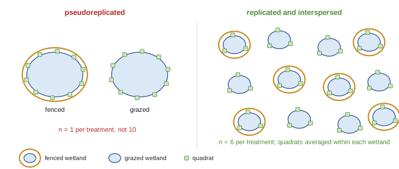
The experimental unit is the smallest unit to which a treatment is independently applied. In the grazing study, the ranch fences whole wetland margins, so the experimental unit is the wetland, not each quadrat within it. If the team places ten quadrats along the edge of one fenced wetland and ten along one unfenced wetland, it has one replicate of each treatment, not ten, because all ten quadrats share whatever makes that particular wetland different: its depth, its soil, its history, the cow that likes to stand in it. Quadrats within a wetland are subsamples. They improve the estimate for that wetland but tell you nothing about variation among wetlands, which is the variation a treatment effect must be judged against.
Replication, applying each treatment to several independent units, does two jobs. It lets you estimate the natural variation among units, without which no test is possible, and it reduces the chance that a treatment effect is really the peculiarity of one unit. How many replicates you need depends on that variation and on the size of effect you want to detect, as shown later in this lesson. In field ecology, replicates are expensive because each may be a separate wetland, lake, forest stand or pasture, and the temptation to substitute subsamples for replicates is strong. Resisting it is the single most important design discipline in the field.
Controls and randomization
A control is a unit that experiences everything the treated units do except the treatment. In the grazing study, control wetlands are grazed season-long as before. Controls must be measured at the same times and in the same way as treated units, because many things change over a season or between years. Sometimes the treatment itself has side effects that need their own control. Fences provide perches for birds and shade and change snow drifting; a procedural control, such as a fence with gaps that cattle can walk through, can separate the effect of excluding cattle from the effect of the fence itself.
Randomization means using a random process, such as a random number generator, to decide which units get which treatment. It protects against conscious and unconscious bias in choosing units, such as fencing the most accessible or the most promising wetlands, and it balances unmeasured confounders on average. It also justifies the statistical test: under the null hypothesis of no effect, every assignment was equally likely, so the observed difference can be compared with the differences produced by all possible assignments, the logic of randomization or permutation tests.
Randomization alone can produce an unlucky layout, with all treated wetlands bunched in one corner of the station. Hurlbert called the goal interspersion: treatments should be spread among each other across the study area so that a spatial gradient, such as a change in soil type from north to south, does not line up with treatment. Restricted randomization, such as randomizing within blocks, achieves both randomness and interspersion.
Blocking
A block is a group of units that are similar to each other, such as wetlands in the same pasture or plots on the same slope. In a randomized complete block design, each treatment is assigned at random to one unit within each block. Because comparisons are made within blocks, variation among blocks is removed from the error, which can greatly increase power when blocks differ a lot. In the grazing study, the twenty-four wetlands lie in six pastures with different soils and stocking histories, so the team pairs wetlands within pastures and randomly fences one of each pair, two pairs per pasture. Block on the strongest known source of variation; if blocks do not differ, blocking costs a few degrees of freedom but little else.
| Design | How treatments are assigned | When to use it | Main risk |
|---|---|---|---|
| Completely randomized | At random among all units | Units are similar and interspersed | Large error variance if units differ |
| Randomized complete block | At random within each block of similar units | Units differ in known ways, such as pasture or slope | Blocks must be chosen before treatment |
| Paired design | One of each pair treated at random | Natural pairs exist, such as adjacent wetlands | Pairs that differ greatly add noise |
| Split-plot | Large-scale factor on whole units, smaller factor within them | Factors operate at different scales, such as grazing on pastures and seeding on plots | Different error terms for each factor |
| BACI | Change occurs at impact units; control units unchanged; both measured before and after | Unplanned or non-random changes such as a development or management shift | Control and impact may differ in trends as well as levels |
Pseudoreplication
In 1984 Stuart Hurlbert reviewed published ecological field experiments and found that a large fraction treated subsamples or repeated measurements as if they were independent replicates. He called this pseudoreplication. Its forms include simple pseudoreplication, with one unit per treatment and many subsamples; sacrificial pseudoreplication, where true replicates exist but their subsamples are pooled into one analysis as if independent; and temporal pseudoreplication, where repeated measurements of the same units over time are treated as independent. The consequence is the same in each case: the variation used to judge the treatment effect is too small, so the test finds effects far more often than it should.
# Pseudoreplication: treating quadrats as replicates inflates false positives.
import numpy as np
from scipy import stats
rng = np.random.default_rng(1984)
def one_study(wetlands_per_trt, quadrats):
    # no true fencing effect; wetlands differ (SD 8 cm), quadrats within a wetland differ (SD 5 cm)
    groups = []
    for trt in range(2):
        means = rng.normal(60, 8, wetlands_per_trt)
        q = means[:, None] + rng.normal(0, 5, (wetlands_per_trt, quadrats))
        groups.append(q)
    p_wrong = stats.ttest_ind(groups[0].ravel(), groups[1].ravel()).pvalue        # quadrats as n
    if wetlands_per_trt < 2:
        return p_wrong < 0.05, None                                                 # no valid test with n = 1
    p_right = stats.ttest_ind(groups[0].mean(1), groups[1].mean(1)).pvalue         # wetland means as n
    return p_wrong < 0.05, p_right < 0.05
for k, q in [(1, 10), (3, 10), (6, 5)]:
    if k == 1:
        res = [one_study(1, q)[0] for _ in range(4000)]
        print(f"{k} wetland per treatment, {q} quadrats: false-positive rate {np.mean(res):.2f} (no valid test exists)")
        continue
    res = np.array([one_study(k, q) for _ in range(4000)])
print(f"{k} wetlands per treatment, {q} quadrats: quadrats-as-replicates {res[:,0].mean():.2f}, wetland means {res[:,1].mean():.2f}")1 wetland per treatment, 10 quadrats: false-positive rate 0.69 (no valid test exists) 3 wetlands per treatment, 10 quadrats: quadrats-as-replicates 0.53, wetland means 0.05 6 wetlands per treatment, 5 quadrats: quadrats-as-replicates 0.35, wetland means 0.05
The simulation has no true fencing effect at all. Analysing wetland means gives the advertised 5 per cent false-positive rate; analysing quadrats as if they were independent rejects the null hypothesis in a large share of studies, because differences among wetlands are mistaken for a treatment effect. With only one wetland per treatment there is no valid test at all, however many quadrats are measured: any difference could be a property of those two wetlands. The cure is to analyse at the level of the experimental unit, either by averaging subsamples within units or by using a mixed model with the unit as a random effect, as lesson 11 explains.
Pseudoreplication is not always avoidable. Whole-lake or whole-watershed experiments often have one treated system, because there is only one lake you are allowed to manipulate. The honest response is to use other designs, such as long time series before and after treatment, and to state clearly that the inference is about that system, rather than to dress up subsamples as replicates.
Before–after–control–impact designs
Many changes ecologists want to study are not under their control and are not randomized: a dam, a pipeline, a wind farm, a new grazing system, a wildfire. A simple comparison of impact and control sites after the change confounds the effect with any pre-existing difference; a simple before-and-after comparison at the impact site confounds it with anything else that changed over the same period, such as a wet year. The before–after–control–impact (BACI) design measures both control and impact sites both before and after the change. The effect is estimated as the change at impact sites minus the change at control sites, the same logic economists call difference-in-differences.
The BACI estimate removes fixed differences between sites and changes common to all sites. Its key assumption is parallel trends: without the change, impact and control sites would have changed by the same amount. Replicating control sites, and ideally impact sites, guards against one control site behaving strangely; measuring in several years before and after, rather than one of each, separates a real effect from year-to-year noise. Designs with multiple controls and multiple sampling times are sometimes called beyond-BACI designs, after work by Underwood in the early 1990s.
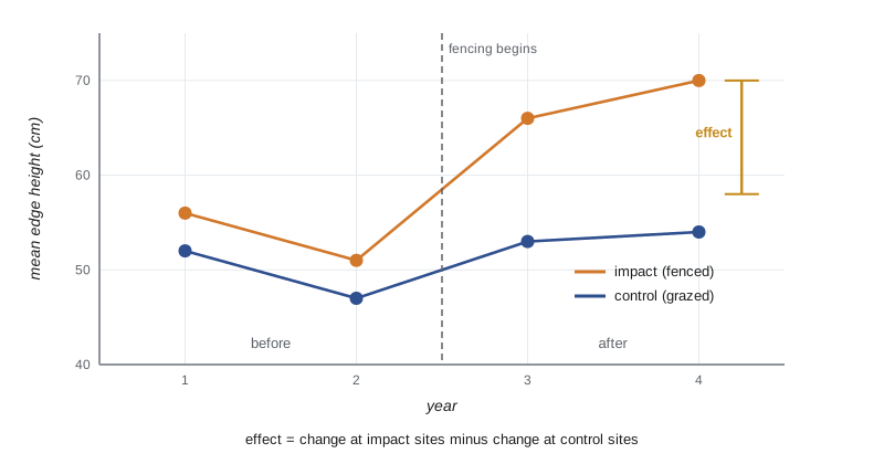
In the grazing study, the ranch decided which wetlands to fence, so the design is a BACI rather than a randomized experiment. The team has two years of measurements before fencing and will collect two years after it, on twelve fenced and twelve unfenced wetlands. They also recorded water depth, soil texture and pasture stocking rate, so they can check whether fenced and unfenced wetlands had similar trends before the change, the only evidence available for the parallel-trends assumption.
Power analysis
Statistical power is the probability that a study will detect an effect of a given size if it exists. It depends on four things: the effect size, the variability among units, the number of replicates and the significance level. Low power is endemic in field ecology, and an underpowered study is worse than wasteful: it is likely to report no effect when there is one, and the effects it does report as significant tend to be exaggerated, because only unusually large estimates pass the threshold. Power analysis before a study tells you how many units you need; done afterwards on the observed effect, it tells you nothing new, so do it in advance.
For simple designs, formulas exist. For realistic field designs, with blocks, repeated years and subsamples, simulation is easier and more honest: write code that generates fake data with the structure you expect, including variation among wetlands, among years and among quadrats, add an effect of the size you care about, analyse it exactly as you plan to analyse the real data, and repeat thousands of times. The fraction of simulated studies that detect the effect is the power. Variance estimates come from pilot data or published studies.
# Power of a BACI design by simulation: how many wetlands per group?
import numpy as np
from scipy import stats
rng = np.random.default_rng(7)
def baci_power(n_sites, effect=10.0, sims=2000):
    hits = 0
    for _ in range(sims):
        site = rng.normal(0, 9, 2 * n_sites)               # persistent wetland differences (cm)
        year = rng.normal(0, 4, 4)                         # shared year effects, years 1-4
        y = 55 + site[:, None] + year[None, :] + rng.normal(0, 6, (2 * n_sites, 4))
        impact = np.arange(2 * n_sites) < n_sites
        y[impact, 2:] += effect                            # fencing raises height after year 2
        change = y[:, 2:].mean(1) - y[:, :2].mean(1)       # after minus before, per wetland
        p = stats.ttest_ind(change[impact], change[~impact]).pvalue
        hits += p < 0.05
    return hits / sims
for n in (4, 6, 8, 12, 16):
    print(f"{n:2d} impact + {n:2d} control wetlands: power to detect a 10 cm effect = {baci_power(n):.2f}")
print(f"12 + 12 wetlands, 5 cm effect: power = {baci_power(12, effect=5.0):.2f}")4 impact + 4 control wetlands: power to detect a 10 cm effect = 0.51 6 impact + 6 control wetlands: power to detect a 10 cm effect = 0.76 8 impact + 8 control wetlands: power to detect a 10 cm effect = 0.87 12 impact + 12 control wetlands: power to detect a 10 cm effect = 0.98 16 impact + 16 control wetlands: power to detect a 10 cm effect = 0.99 12 + 12 wetlands, 5 cm effect: power = 0.49
With twelve impact and twelve control wetlands, the design has high power to detect a 10-centimetre effect but much less power for a 5-centimetre effect. Note that because the analysis uses each wetland's change from before to after, persistent differences among wetlands cancel out; that is why BACI designs can be powerful even when sites differ a lot. If the team cared about 5-centimetre effects, it would need more wetlands or more years. Power analysis turns a vague hope into an explicit trade-off the team and its funders can discuss.
Practical design checklist
Before the first field day, write down the experimental unit, the treatments and controls, how treatments will be assigned, the blocks, the number of replicates and subsamples and why, what will be measured, when and by whom, and the planned analysis. Check that each treatment has at least three, preferably more, independent replicates; that treatments are interspersed; that observers do not know which units are treated when that is possible, to avoid biased measurements; and that measurements in control and treated units are made in the same order or alternated, so that time of day or observer fatigue does not line up with treatment. A short pilot season tests methods, estimates variances and almost always reveals a problem you did not anticipate.
Worked problem
Spotting the experimental unit
Priya plans to test whether fencing affects seedling survival. She marks 30 seedlings inside one fenced exclosure and 30 outside it, and plans a chi-squared test on 60 seedlings. What is wrong, and how could she fix it?
Show solution
- The treatment, fencing, is applied to the exclosure, so the exclosure is the experimental unit.
- With one fenced and one unfenced area, n = 1 per treatment; the seedlings are subsamples, and the chi-squared test treats them as independent replicates, which is simple pseudoreplication.
- Any difference could arise from the two areas differing in soil, moisture or herbivores other than cattle.
- Fix: use several fenced and unfenced areas, for example six pairs of plots with fencing randomized within each pair, and analyse the proportion surviving per plot, or a mixed model with plot as a random effect.
Answer: The 60 seedlings are subsamples of one unit per treatment; she needs several independently fenced and unfenced plots, randomized and interspersed, analysed at the plot level.
Common mistakes
MistakeCounting quadrats or individuals within a single treated area as replicates.
InsteadIdentify the unit to which the treatment was applied and replicate that unit.
MistakeChoosing which units to treat by convenience.
InsteadRandomize, ideally within blocks, so treatments are unbiased and interspersed.
MistakeComparing impact and control sites only after a change.
InsteadMeasure before as well as after, at both, and estimate the difference in differences.
MistakeRunning a power analysis after a non-significant result using the observed effect.
InsteadPlan power in advance for the smallest effect that matters, using pilot or published variances.
MistakeTreating repeated measurements of the same plots as independent samples.
InsteadAnalyse change per unit or use models that account for repeated measures.
Summary and key terms
- The experimental unit is the unit to which a treatment is independently applied; subsamples within it are not replicates.
- Controls must differ from treated units only in the treatment; procedural controls separate side effects.
- Randomization prevents bias and supports valid tests; blocking and interspersion handle known gradients.
- Pseudoreplication inflates false-positive rates by mistaking variation among units for a treatment effect.
- BACI designs estimate an effect as the difference in changes at impact and control sites, assuming parallel trends.
- Power depends on effect size, variability, replication and alpha; simulation handles realistic designs.
- experimental unit
- The smallest unit to which a treatment is independently applied.
- subsample
- A measurement taken within an experimental unit; not an independent replicate.
- replication
- Applying each treatment to several independent experimental units.
- procedural control
- A control that experiences the side effects of applying a treatment without the treatment itself.
- interspersion
- Spreading treatments among each other across the study area.
- block
- A group of similar units within which treatments are randomized.
- pseudoreplication
- Treating non-independent subsamples or repeated measures as independent replicates.
- BACI design
- A design measuring control and impact units before and after a change.
- parallel trends
- The assumption that impact and control units would have changed equally without the treatment.
- statistical power
- The probability of detecting an effect of a given size if it exists.
Practice problems
Work each problem on paper first, then reveal the answer to check.
Cattle are excluded from whole pastures; grass is clipped in plots within pastures. What are the experimental units for each factor?
Show answer
Pastures for grazing; plots for clipping, a split-plot design.
Name Hurlbert's three main forms of pseudoreplication.
Show answer
Simple, sacrificial and temporal.
Impact wetlands averaged 50 cm before and 62 cm after; controls averaged 47 cm before and 51 cm after. What is the BACI estimate?
Show answer
(62 - 50) - (51 - 47) = 12 - 4 = 8 cm.
What assumption makes that estimate valid?
Show answer
Parallel trends: without fencing, impact wetlands would have changed as much as controls.
Why does blocking by pasture increase power?
Show answer
It removes variation among pastures from the error used to test the treatment.
What is a procedural control for a fence?
Show answer
A fence with gaps that lets cattle through, so fence side effects occur without exclusion.
List the four quantities that determine power.
Show answer
Effect size, variability, sample size and significance level.
Why are significant results from underpowered studies often exaggerated?
Show answer
Only unusually large estimates reach significance when power is low.
Lesson quiz · 5 questions
Score 60% or more to complete this lesson.
Create a free account to save your progress, take quizzes and earn a certificate.