
BIOL-430 · Lesson 5 of 12 · 24 min
Estimating abundance I: plots, transects and distance sampling
How many are there? Few questions in ecology are as basic, and few are as hard to answer well. Abundance, the number of individuals in a defined area, and density, the number per unit area, drive population models, harvest quotas, species-at-risk assessments and evaluations of management. This lesson covers methods that count organisms in plots or along lines: complete counts, quadrat counts and their statistics, and distance sampling, which corrects line and point counts for animals that are present but missed. Lesson 6 turns to methods based on marked individuals and repeated surveys.
Complete counts and censuses
For some populations a complete count is possible: every nest in a small seabird colony, every tree in a plot, every breeding pair of a conspicuous species on a small island. Such censuses are valuable, but true completeness is rarer than it looks. Aerial waterfowl surveys, such as the long-running cooperative surveys of breeding ducks across the prairie pothole region, count only a strip below the aircraft and correct for birds missed using ground counts on a subset of segments. Winter counts of deer from helicopters miss animals under conifers. Whenever a count is called a census, ask how missed individuals were handled.
Quadrat counts
When organisms are counted in randomly placed plots of known area, density is estimated by the mean count divided by plot area, and abundance by multiplying density by the total area. If the plots are a random sample, the standard error of the mean count divided by plot area gives the standard error of density. The spatial pattern of the organisms matters for precision. If individuals are placed independently at random, counts per quadrat follow a Poisson distribution, whose variance equals its mean. Most organisms are clumped, with more empty quadrats and more crowded ones than a Poisson distribution predicts, so the variance exceeds the mean. A few, such as territorial animals or competing desert shrubs, are more regular than random, with variance below the mean.
The variance-to-mean ratio, sometimes called the index of dispersion, is a quick diagnostic: values near 1 suggest randomness, above 1 clumping and below 1 regularity. Under randomness, \((n-1) s^2 / \bar{x}\) follows approximately a chi-squared distribution with \(n-1\) degrees of freedom, which gives a test. Clumped counts are often well described by a negative binomial distribution, with variance \(\mu + \mu^2/k\); small values of the aggregation parameter \(k\) mean strong clumping. Clumping matters for design: clumped populations need more quadrats for the same precision, and the negative binomial reappears in lesson 11 as the standard model for overdispersed counts.
# Quadrat counts of sedge flowering stems: density, CI and dispersion.
import numpy as np
from scipy import stats
rng = np.random.default_rng(55)
area = 0.25                                         # 0.5 m x 0.5 m quadrats
counts = rng.negative_binomial(n=1.5, p=1.5 / (1.5 + 6.0), size=60)   # clumped, mean 6
m, s2, n = counts.mean(), counts.var(ddof=1), len(counts)
se = np.sqrt(s2 / n)
t = stats.t.ppf(0.975, n - 1)
print(f"mean count {m:.2f} per quadrat, variance {s2:.2f}, variance-to-mean ratio {s2 / m:.2f}")
chi = (n - 1) * s2 / m
print(f"dispersion test: chi2 = {chi:.0f} on {n - 1} df, p = {stats.chi2.sf(chi, n - 1):.1e} (clumped)")
print(f"density = {m / area:.1f} stems/m2, 95% CI {(m - t * se) / area:.1f} to {(m + t * se) / area:.1f}")
k = m**2 / (s2 - m)
print(f"moment estimate of negative binomial k = {k:.2f}")
for target in (0.2, 0.1):
    nreq = (1 / m + 1 / k) / target**2
print(f"quadrats needed for SE = {target:.0%} of the mean: about {nreq:.0f}")mean count 7.93 per quadrat, variance 46.64, variance-to-mean ratio 5.88 dispersion test: chi2 = 347 on 59 df, p = 2.3e-42 (clumped) density = 31.7 stems/m2, 95% CI 24.7 to 38.8 moment estimate of negative binomial k = 1.63 quadrats needed for SE = 20% of the mean: about 19 quadrats needed for SE = 10% of the mean: about 74
The last lines use a standard result for the negative binomial: the number of quadrats needed for the standard error to be a fraction \(D\) of the mean is about \((1/\bar{x} + 1/k)/D^2\). Halving the target relative error quadruples the effort. Such calculations, done with pilot data, are how monitoring programs choose sample sizes.
Line and point counts
For mobile animals, such as birds in grassland, counting along a line or at a point is faster than searching plots. An observer walks a transect or stands at a point for a fixed time, often 5 to 10 minutes for songbirds, and records every individual seen or heard. Point counts are the backbone of large bird monitoring programs, including the North American Breeding Bird Survey, run jointly by the United States Geological Survey and the Canadian Wildlife Service since 1966, in which volunteers stop at 50 points along a roadside route each June. Such counts give an index of abundance useful for tracking trends, provided detection probability does not change over time, an assumption that is reasonable for some species and not for others.
Fixed-radius counts record only individuals within, say, 50 or 100 metres of the observer, which converts counts into densities if everything within the radius is detected. That is rarely true for wide radii. Distance sampling, developed in its modern form by Buckland, Anderson, Burnham and colleagues from the 1970s on, solves the problem by recording the distance to each detected animal and using the decline in detections with distance to estimate how many were missed.
Distance sampling
The key assumption of distance sampling is that animals on the line or at the point are detected with certainty, and that detection probability declines with distance in a smooth way described by a detection function \(g(x)\), with \(g(0) = 1\). A common choice is the half-normal function:
For line transects, if \(w\) is the truncation distance beyond which detections are ignored, the average detection probability within the strip is \(P_a = \frac{1}{w}\int_0^w g(x)\,dx\), and the effective strip half-width is \(\mu = \int_0^w g(x)\,dx\). Density is then estimated as
where \(n\) is the number of animals detected and \(L\) the total transect length. For point counts, detection area grows with distance, so the distribution of detection distances is weighted by distance, and density is \(n/(k \pi \rho^2)\), where \(k\) is the number of points and \(\rho\) the effective detection radius. The estimation uses only the shape of the distribution of detection distances, which is why accurate distances matter: rounding to convenient values, such as 50 or 100 metres, and moving animals before they are detected both bias estimates. Laser rangefinders help with distance measurement.
Other assumptions are that animals are detected at their initial location, before any movement in response to the observer; that distances are measured accurately; and that detections are independent or, for groups, that group size is recorded. Clusters, such as flocks, are treated as the unit of detection and density of individuals is the density of clusters times mean cluster size. Distance software, notably the Distance program developed at the University of St Andrews and its R packages, fits detection functions with adjustment terms and covariates such as observer or vegetation height.
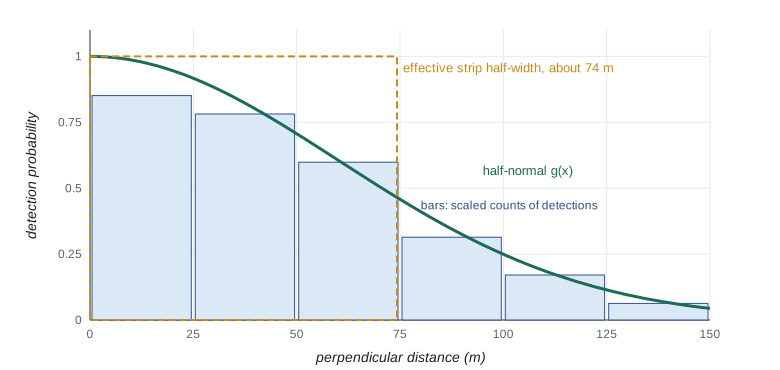
# Line-transect distance sampling for savannah sparrows (synthetic): half-normal fit by maximum likelihood.
import numpy as np
from scipy import optimize, special
rng = np.random.default_rng(301)
L, w = 20_000.0, 150.0            # 20 km of transects, truncate at 150 m
true_D, sigma = 0.00015, 60.0      # 1.5 birds per ha = 0.00015 per m2
N_strip = rng.poisson(true_D * 2 * L * w)
x = rng.uniform(0, w, N_strip)
seen = rng.uniform(size=N_strip) < np.exp(-x**2 / (2 * sigma**2))
d = x[seen]
def mu(s):  # integral of half-normal from 0 to w
    return s * np.sqrt(np.pi / 2) * special.erf(w / (s * np.sqrt(2)))
def nll(log_s):
    s = np.exp(log_s)
    return -(np.sum(-d**2 / (2 * s**2)) - len(d) * np.log(mu(s)))
fit = optimize.minimize_scalar(nll, bounds=(1, 7), method='bounded')
s_hat = np.exp(fit.x)
D_hat = len(d) / (2 * L * mu(s_hat))
naive = len(d) / (2 * L * w)
print(f"detections: {len(d)} of {N_strip} birds in the strip")
print(f"sigma = {s_hat:.1f} m, effective strip half-width = {mu(s_hat):.1f} m, P_a = {mu(s_hat) / w:.2f}")
print(f"density: distance estimate {D_hat * 1e4:.1f} per ha, naive strip count {naive * 1e4:.1f} per ha, true {true_D * 1e4:.1f}")detections: 433 of 891 birds in the strip sigma = 60.7 m, effective strip half-width = 75.0 m, P_a = 0.50 density: distance estimate 1.4 per ha, naive strip count 0.7 per ha, true 1.5
The naive estimate, which assumes every bird within 150 metres was detected, falls well short of the truth because detection drops steeply with distance. The distance estimate recovers it. Precision comes from two sources: the encounter rate, \(n/L\), which varies among transects and is usually the larger source, and the estimate of the detection function. Variance is therefore estimated using transects as replicates, with the detection function uncertainty added.
Covariates, observers and habitat
Detection probability often depends on things other than distance: observer skill, wind and noise, time of morning, singing rate, vegetation height and density. Multiple-covariate distance sampling includes such variables in the scale parameter \(\sigma\). In the grazing study this is essential. If fenced wetlands develop taller vegetation, sparrows may be detected over shorter distances there, and counts without correction would understate any increase. With vegetation height recorded at each point, the detection function can differ between treatments while the density estimate remains comparable.
| Method | Data recorded | Key assumptions | Best for |
|---|---|---|---|
| Quadrat count | Counts in plots of known area | Everything in a plot is found; plots random | Plants, sessile or slow animals |
| Fixed-radius point count | Counts within a set radius | Everything within the radius detected | Indices of songbird abundance |
| Line-transect distance sampling | Perpendicular distance to each detection | Certain detection on the line, no responsive movement, accurate distances | Birds and mammals in open habitat, ungulates, dolphins |
| Point-transect distance sampling | Radial distance from the point | Certain detection at the point, as above | Songbirds in patchy or forested habitat |
| Strip transect with correction | Counts in a strip plus detection-rate subsample | Correction factor transferable across strips | Aerial waterfowl and ungulate surveys |
Other count-based methods
Removal of the observer's influence is one challenge; another is availability. A bird that does not sing during a five-minute count is unavailable for detection even if it is close. Time-removal methods divide the count into intervals and treat the first detection of each individual as a removal, estimating the probability of singing at least once. Combining time-removal and distance data, as the Boreal Avian Modelling Project in Canada has done to integrate point counts from many studies across the boreal forest, separates availability from perceptibility. Double-observer methods, in which two observers count independently, estimate detection probability from the overlap in their records, much like a two-sample mark–recapture study.
Indices, such as pellet counts for deer, track counts in snow, calls per hour for frogs or captures per trap-night, are cheaper than absolute estimates. They are useful when the relationship between index and abundance is constant across the comparisons you make, which must be argued rather than assumed. Calibrating an index against absolute estimates on a subset of sites, a double sampling design, makes it more defensible.
Worked problem
Computing a line-transect density by hand
Sam walked 8 km of transects and detected 120 savannah sparrows. A half-normal detection function fitted to the distances gives an effective strip half-width of 55 m. Estimate density per hectare and compare with a naive estimate that assumes all birds within 100 m were detected.
Show solution
- Area effectively searched = 2 x L x mu = 2 x 8,000 x 55 = 880,000 m2 = 88 ha.
- Distance-sampling density = 120 / 88 = 1.36 birds per hectare.
- Naive area = 2 x 8,000 x 100 = 1,600,000 m2 = 160 ha, giving 120 / 160 = 0.75 per hectare.
- The naive estimate is about 45 per cent too low because many birds between 55 and 100 m were missed.
Answer: About 1.4 birds per hectare from distance sampling, against 0.75 from the naive strip count.
Common mistakes
MistakeAssuming quadrat counts are Poisson when the organism is clumped.
InsteadCheck the variance-to-mean ratio; use negative binomial methods and plan for more quadrats.
MistakeRounding detection distances to 25 or 50 m.
InsteadMeasure distances accurately, ideally with a rangefinder, and record them before animals move.
MistakeUsing individual detections as replicates for variance.
InsteadUse transects or points as replicates for the encounter rate.
MistakeComparing raw counts between habitats with different visibility.
InsteadModel detection with distance and covariates such as vegetation height.
MistakeCalling an index an estimate of abundance.
InsteadReport it as an index, and calibrate it against absolute estimates where possible.
Summary and key terms
- Density is the number per unit area; abundance multiplies density by area.
- Quadrat counts of random organisms are Poisson; clumped organisms have variance above the mean and need more quadrats.
- Point and line counts are efficient but confound abundance with detection unless distances or other data are collected.
- Distance sampling models detection as a function of distance and estimates density from the effective strip half-width or detection radius.
- Key assumptions are certain detection at zero distance, no responsive movement and accurate distances.
- Covariates, time-removal and double-observer methods handle variation in detection and availability.
- density
- The number of individuals per unit area.
- index of dispersion
- The variance-to-mean ratio of counts, used to diagnose random, clumped or regular patterns.
- negative binomial distribution
- A distribution for overdispersed counts with variance greater than the mean.
- point count
- A survey in which an observer records all individuals detected from a fixed point for a set time.
- distance sampling
- Estimating density by modelling how detection probability declines with distance from a line or point.
- detection function
- The probability of detecting an animal as a function of its distance from the observer.
- effective strip half-width
- The distance at which a strip with perfect detection would produce the same expected count.
- truncation distance
- The distance beyond which detections are excluded from analysis.
- availability
- The probability that an animal presents a cue, such as song, during a survey.
- double sampling
- Calibrating a cheap index against an accurate method on a subset of units.
Practice problems
Work each problem on paper first, then reveal the answer to check.
Quadrat counts have mean 4 and variance 4.2. What pattern is suggested?
Show answer
Approximately random (variance-to-mean ratio about 1).
What does a small negative binomial k indicate?
Show answer
Strong clumping.
In a point-count survey, why are detections weighted by distance?
Show answer
The area at distance r grows with r, so more animals are available at greater distances.
A survey of 10 km of transects detects 80 animals; the effective strip half-width is 40 m. Estimate density per km2.
Show answer
80 / (2 x 10 x 0.04) = 100 per km2.
Why must animals be detected before they move in response to the observer?
Show answer
Movement away biases distances upward or toward zero, distorting the detection function.
Name two ways to deal with birds that do not sing during a count.
Show answer
Time-removal models and double-observer methods.
What is the main source of variance in most distance-sampling estimates?
Show answer
Variation in encounter rate among transects.
Why include vegetation height as a covariate in the grazing study?
Show answer
Fencing may change vegetation height and therefore detectability, biasing comparisons.
Lesson quiz · 5 questions
Score 60% or more to complete this lesson.
Create a free account to save your progress, take quizzes and earn a certificate.