
BIOL-420 · Lesson 11 of 12 · 27 min
Tools of modern neuroscience and computational models
Progress in neuroscience has repeatedly followed new tools: the Golgi stain, the microelectrode, the patch clamp, functional imaging. The last two decades have brought another transformation. Neuroscientists can now record from thousands of neurons at once, switch genetically defined cell types on and off with light, read out calcium in single synapses in behaving animals, and reconstruct every synapse in a cubic millimetre of cortex. At the same time, computational models have grown from single neurons to networks that can be compared with recordings. This lesson surveys how brain activity is measured and manipulated, what each method can and cannot tell us, how complete wiring diagrams are being built, and how simple models such as attractor networks capture memory and computation. A case study of hunger circuits in the hypothalamus shows the tools working together.
Measuring activity in humans
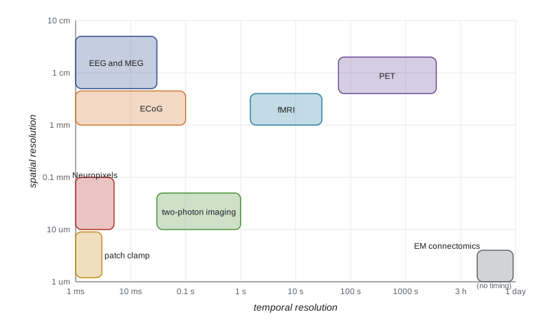
Non-invasive methods trade spatial for temporal resolution. Electroencephalography (EEG) records voltage at the scalp produced by synchronized synaptic currents in large populations of cortical pyramidal neurons aligned in parallel. It has millisecond resolution but centimetre-scale spatial blurring because the skull smears currents, and it is dominated by rhythms such as alpha (8 to 12 hertz) over the visual cortex when the eyes are closed. Event-related potentials, averaged over many trials, reveal the timing of sensory and cognitive processing. Magnetoencephalography (MEG) measures the tiny magnetic fields of the same currents, less distorted by the skull, using superconducting sensors or, more recently, optically pumped magnetometers that can be worn.
Functional magnetic resonance imaging (fMRI) measures the blood-oxygen-level-dependent (BOLD) signal. Active neurons increase local blood flow more than oxygen consumption, so deoxygenated hemoglobin, which is paramagnetic, falls, and the MRI signal rises. The BOLD response is an indirect, slow measure of activity: it peaks about 5 to 6 seconds after a brief neural event, reflects synaptic input and local processing more than spiking output, and resolves millimetre-scale voxels, each containing hundreds of thousands of neurons. It cannot distinguish excitation from inhibition, both of which consume energy. Its strengths are whole-brain coverage in healthy people and the ability to relate activity to cognition.
fMRI analysis has known pitfalls. Because tens of thousands of voxels are tested, false positives accumulate unless corrected for multiple comparisons; a famous 2009 poster reported apparent activation in a dead salmon shown pictures of people, to make that point. Circular analysis, selecting voxels with one contrast and then testing them with the same data, inflates effects. A 2016 study found that some widely used cluster-correction methods produced far more false positives than assumed. Small sample sizes also make brain-wide association studies unreliable: a 2022 analysis of about 50,000 participants showed that linking individual differences in brain structure or function to behaviour or mental health needs thousands of participants. These lessons led to preregistration, open data and much larger studies.
Invasive recordings in humans are possible when clinically justified. Patients with drug-resistant epilepsy often have electrodes placed on the cortical surface (electrocorticography) or in deep structures for days to locate seizure origins, and many volunteer for research, providing single-neuron and local field recordings from the human hippocampus, amygdala and cortex (lesson 10). Recordings during deep brain stimulation surgery and from brain–computer interface participants (lesson 12) add further data.
Recording many neurons in animals
Single extracellular electrodes, since the 1950s, gave the foundational discoveries of receptive fields, place cells and dopamine prediction errors, but recorded one or a few neurons at a time. Multi-electrode arrays changed the scale. Neuropixels probes, silicon shanks about 1 centimetre long with nearly a thousand recording sites, introduced in 2017, let researchers record hundreds of neurons across several brain regions simultaneously in behaving mice; a 2019 study recorded about 30,000 neurons across 42 brain regions of mice performing a choice task, finding that action-related signals were widespread across the brain. Spike sorting algorithms assign each recorded spike to a neuron using its waveform across neighbouring sites. Recordings of such size revealed that population activity often lies on low-dimensional structures, the neural manifolds mentioned in lesson 9, and that brain-wide activity is strongly modulated by movement and arousal.
Optical recording offers cell-type specificity. Genetically encoded calcium indicators such as GCaMP, a fusion of green fluorescent protein and calmodulin whose fluorescence rises when calcium binds, report spiking activity through the calcium that enters with each action potential. Two-photon microscopy, in which fluorescence is excited only at the focal point by near-simultaneous absorption of two infrared photons, images cells hundreds of micrometres deep in living brain with little scattering. Researchers can watch thousands of neurons, identified by their genes, over days and weeks as an animal learns, and can image individual dendritic spines. Miniature head-mounted microscopes allow imaging in freely moving animals. Calcium signals are slow relative to spikes, so voltage indicators, fluorescent proteins that report membrane potential directly, are being developed for millisecond resolution. Fluorescent sensors for dopamine, acetylcholine, serotonin and other transmitters, built from their receptors, now let researchers watch neuromodulator release in real time.
Manipulating activity: optogenetics and chemogenetics
Correlation is not causation. To test whether a neuron population causes a behaviour, one must change its activity. Optogenetics, developed by Edward Boyden, Karl Deisseroth and colleagues in 2005, introduces light-sensitive microbial proteins into genetically chosen neurons. Channelrhodopsin-2, a light-gated cation channel from the green alga Chlamydomonas, depolarizes neurons within milliseconds when illuminated with blue light; halorhodopsin, a chloride pump, and archaerhodopsin, a proton pump, silence neurons with yellow or green light; and newer channels respond to red light, which penetrates tissue more deeply. Genetic targeting usually uses mice that express Cre recombinase in a cell type of interest, combined with a virus carrying a Cre-dependent opsin gene, so only that cell type becomes light-sensitive. Optical fibres deliver light deep into the brain. Optogenetics was used to show that stimulating dopamine neurons is rewarding, that dentate gyrus engram cells can drive recall (lesson 10) and that specific hypothalamic neurons drive feeding.
Chemogenetics uses engineered receptors activated only by otherwise inert designer drugs. DREADDs (designer receptors exclusively activated by designer drugs), developed by Bryan Roth's group from muscarinic receptors in 2007, can excite (hM3Dq) or inhibit (hM4Di) neurons for hours after a systemic injection. Chemogenetics is slower and less precise in time than optogenetics but needs no implanted fibre and affects a whole population for long periods. A complication was discovered in 2017: the original ligand, clozapine-N-oxide, is converted to clozapine, which acts on native receptors, so newer ligands and careful controls are now used.
Both approaches have limits. Artificially synchronous stimulation differs from natural activity, silencing a region can cause effects in distant regions that are mistaken for direct effects, and behaviour can compensate after chronic manipulations. Combining manipulation with simultaneous recording, and stimulating patterns that mimic natural activity, addresses some of these concerns. Optogenetics has begun to reach the clinic: in 2021 a man with retinitis pigmentosa recovered partial vision after a light-sensitive protein was delivered to his retinal ganglion cells, used with special goggles.
| Method | What it measures or does | Strengths | Main limitations |
|---|---|---|---|
| EEG and MEG | Population synaptic currents at the scalp | Millisecond timing, non-invasive | Poor spatial resolution, mainly cortex |
| fMRI (BOLD) | Blood oxygenation linked to activity | Whole brain, millimetre voxels, non-invasive | Slow, indirect, many statistical pitfalls |
| Neuropixels and electrode arrays | Spikes of hundreds of single neurons | Millisecond timing, many regions | Invasive, limited cell-type identification |
| Two-photon calcium imaging | Calcium in genetically defined cells | Cell-type specific, tracks cells over weeks | Slow relative to spikes, limited depth |
| Optogenetics | Excites or silences cells with light | Millisecond control of defined cell types | Needs light delivery, unnatural synchrony |
| Chemogenetics (DREADDs) | Excites or silences cells with a designer drug | Long-lasting, no implant needed | Slow, ligand off-target effects |
| Electron microscopy connectomics | Every synapse in a volume | Complete wiring at nanometre resolution | Static, enormous data, small volumes |
Connectomics
A connectome is the complete wiring diagram of a nervous system. The first, for C. elegans, was reconstructed by hand from serial electron micrographs and published by John White, Sydney Brenner and colleagues in 1986. It took decades for the methods to scale. Serial-section electron microscopy now images brain tissue at a few nanometres per pixel, and machine-learning segmentation, checked and corrected by human proofreaders, traces every neuron and synapse. In October 2024 the FlyWire consortium published the complete connectome of an adult fruit fly brain: about 139,000 neurons and about 50 million synapses, with thousands of cell types annotated; models built from it predicted which neurons would respond to tastes and drive feeding. In April 2025 the MICrONS project published a functional connectome of about a cubic millimetre of mouse visual cortex, containing roughly 200,000 cells and around half a billion synapses, in which the same neurons had been imaged with calcium indicators while the mouse viewed visual stimuli before the tissue was processed, linking function to structure. A complete mouse brain, about 500 times larger, is a goal for the coming decade; a human brain, a thousand times larger again, remains far off.
Connectomes are necessary but not sufficient for understanding circuits. They omit neuromodulators, electrical synapse strengths in many cases, synaptic weights and dynamics, and they are snapshots of one individual. Still, they constrain models powerfully: the fly connectome revealed how heading direction is computed in a ring-shaped network in the central complex, matching predictions of attractor models described next.
Computational models: from neurons to networks
Models in neuroscience range from detailed simulations to abstract networks. The integrate-and-fire neuron of lesson 2 and compartmental models of lesson 3 describe single cells. Rate models describe a population's average firing rate \(r\), with dynamics such as \(\tau \, dr/dt = -r + f(\sum w\, r_{\text{in}} + I)\), where \(f\) is a nonlinear activation function. Networks of excitatory and inhibitory populations show balanced states in which large excitatory and inhibitory inputs nearly cancel, producing irregular firing like that observed in cortex, and they generate oscillations whose frequency depends on the time constants of inhibition. Gamma oscillations (30 to 80 hertz), for example, arise from interactions between pyramidal cells and fast-spiking interneurons.
Attractor networks store memories as stable patterns of activity. In 1982 John Hopfield described a network of binary neurons with symmetric connections set by a Hebbian rule, \(w_{ij} \propto \sum_\mu \xi_i^\mu \xi_j^\mu\), where \(\xi^\mu\) are stored patterns. Each stored pattern becomes a minimum of an energy function; starting from a corrupted version, the network's dynamics descend to the nearest minimum, completing the pattern. A Hopfield network of \(N\) neurons can reliably store about \(0.14N\) random patterns before memories interfere. The model gave a precise meaning to content-addressable memory and pattern completion, the function proposed for hippocampal CA3 (lesson 10). Hopfield and Geoffrey Hinton, who extended these ideas to Boltzmann machines and later to deep learning, shared the 2024 Nobel Prize in Physics.
# Hopfield network: store patterns with a Hebbian rule and recall them from corrupted cues.
import numpy as np
rng = np.random.default_rng(12)
N = 200
def train(patterns):
    W = sum(np.outer(p, p) for p in patterns) / N
    np.fill_diagonal(W, 0)
    return W
def recall(W, s, sweeps=10):
    s = s.copy()
    for _ in range(sweeps):
        for i in rng.permutation(N):           # asynchronous updates
            s[i] = 1 if W[i] @ s >= 0 else -1
    return s
def test(n_patterns, flip=0.25, trials=5):
    pats = [rng.choice([-1, 1], N) for _ in range(n_patterns)]
    W = train(pats)
    overlaps = []
    for _ in range(trials):
        k = rng.integers(n_patterns)
        cue = pats[k].copy()
        idx = rng.choice(N, int(flip * N), replace=False)
        cue[idx] *= -1                         # corrupt 25 per cent of the bits
        out = recall(W, cue)
        overlaps.append(out @ pats[k] / N)
    return np.mean(overlaps)
print("cue overlap with stored pattern: 0.50 (25% of units flipped)")
for P in (5, 10, 20, 28, 40, 60):
print(f"{P:3d} patterns (load {P/N:.2f}): overlap after recall = {test(P):.2f}")cue overlap with stored pattern: 0.50 (25% of units flipped) 5 patterns (load 0.03): overlap after recall = 1.00 10 patterns (load 0.05): overlap after recall = 1.00 20 patterns (load 0.10): overlap after recall = 1.00 28 patterns (load 0.14): overlap after recall = 0.52 40 patterns (load 0.20): overlap after recall = 0.38 60 patterns (load 0.30): overlap after recall = 0.33
Below its capacity the network restores patterns almost perfectly from cues with a quarter of the units wrong; as the load approaches and passes about 0.14N, recall degrades because stored patterns interfere and spurious attractors appear. Continuous attractor networks extend the idea to represent continuous variables: a ring of neurons with local excitation and broad inhibition can hold a bump of activity at any position, representing heading direction, as found in the fly central complex and the mammalian head direction system, and two-dimensional versions model grid cells.
Modern work also compares artificial neural networks trained on tasks with the brain. Networks trained to recognize objects develop representations resembling the primate ventral stream (lesson 7), networks trained on reaching develop dynamics resembling motor cortex (lesson 9), and recurrent networks trained on navigation develop grid-like units. Such task-trained models are hypotheses about what computations a region performs, testable against recordings, but they differ from brains in learning rules, architecture and energy use: a human brain runs on about 20 watts.
A case study: hunger circuits
The hypothalamus regulates feeding, drinking, temperature, reproduction and stress. Research on hunger shows how the modern tools combine. Neurons in the arcuate nucleus that express agouti-related peptide (AgRP) are activated by fasting and by the stomach hormone ghrelin and inhibited by the fat-derived hormone leptin; neighbouring POMC neurons do the reverse. In 2011 Scott Sternson's and Bradford Lowell's groups showed with optogenetics and chemogenetics that activating AgRP neurons makes fed mice eat voraciously within minutes, and silencing them reduces eating. Calcium imaging and fibre photometry then revealed a surprise: AgRP neuron activity falls within seconds when a hungry mouse merely sees or smells food, before eating, so these neurons anticipate the consequences of eating rather than simply tracking energy deficit. Their activity feels unpleasant, which mice work to end, suggesting that hunger motivates partly through negative feelings. Similar studies of thirst neurons in the lamina terminalis showed that drinking is anticipated by signals from the mouth and throat. Clinically, hormones of the gut–brain axis, such as glucagon-like peptide-1 (GLP-1), act on brainstem and hypothalamic circuits, and drugs that mimic GLP-1 have become major treatments for obesity and type 2 diabetes.
Worked problem
Choosing a method for a question
An invented research group asks whether parvalbumin-expressing interneurons in mouse visual cortex are necessary for orientation selectivity in pyramidal neurons. Design an experiment, naming the measurement and manipulation tools.
Show solution
- Target the cell type genetically: use mice expressing Cre in parvalbumin neurons and inject a Cre-dependent inhibitory opsin, such as an archaerhodopsin or a light-gated chloride channel, into visual cortex.
- Measure pyramidal neuron tuning: express a calcium indicator such as GCaMP in pyramidal neurons (using a different promoter) and image with two-photon microscopy while presenting oriented gratings.
- Compare tuning curves with and without light on interleaved trials, so each neuron serves as its own control, and include light-only control animals without opsin.
- Interpret cautiously: silencing may change overall activity levels, so test whether tuning width changes beyond what a simple change in gain would produce.
Answer: Cre-dependent optogenetic silencing of parvalbumin interneurons combined with two-photon calcium imaging of pyramidal tuning, with interleaved and opsin-free controls.
Common mistakes
MistakeTreating the BOLD signal as a direct measure of spiking.
InsteadBOLD is a slow hemodynamic signal that reflects synaptic input and local processing more than output spikes.
MistakeReporting fMRI results without correcting for multiple comparisons.
InsteadTesting many voxels guarantees false positives unless corrected.
MistakeConcluding that a region computes a function because silencing it changes behaviour.
InsteadSilencing can act through downstream effects or disrupt unrelated processes; complementary evidence is needed.
MistakeAssuming a connectome reveals how a circuit works.
InsteadWiring diagrams omit dynamics, neuromodulation and synaptic weights; they constrain but do not determine function.
MistakeExpecting a Hopfield network to store unlimited memories.
InsteadCapacity is about 0.14N random patterns; beyond it, memories interfere.
Summary and key terms
- EEG and MEG offer millisecond timing; fMRI offers whole-brain millimetre maps of a slow hemodynamic signal with known statistical pitfalls.
- Neuropixels probes record hundreds of neurons across regions; calcium and transmitter sensors image defined cells and signals.
- Optogenetics and chemogenetics manipulate genetically defined neurons to test causality, each with limitations.
- Electron microscopy connectomes now cover a whole fly brain and a cubic millimetre of mouse cortex.
- Rate, balanced and attractor models describe network dynamics; Hopfield networks store about 0.14N patterns.
- Combined tools revealed that hunger neurons anticipate food and motivate through negative feelings.
- BOLD signal
- The fMRI signal reflecting changes in blood oxygenation linked to neural activity.
- event-related potential
- An averaged EEG response time-locked to a stimulus or event.
- Neuropixels probe
- A silicon probe with hundreds of recording sites for large-scale single-neuron recording.
- calcium indicator
- A fluorescent protein or dye whose brightness reports intracellular calcium.
- two-photon microscopy
- Fluorescence microscopy using simultaneous absorption of two photons for deep, focal imaging.
- optogenetics
- Control of genetically defined neurons with light-sensitive proteins.
- chemogenetics
- Control of neurons with engineered receptors activated by designer drugs.
- Cre recombinase
- An enzyme used to restrict gene expression to cell types that express it.
- attractor network
- A network whose dynamics settle into stable activity patterns that can represent memories.
- Hopfield network
- A recurrent network with symmetric Hebbian weights that performs pattern completion.
Practice problems
Work each problem on paper first, then reveal the answer to check.
Why does EEG have poor spatial resolution?
Show answer
The skull and scalp blur the electrical fields of underlying cortical currents.
About how long after a brief neural event does the BOLD response peak?
Show answer
About 5 to 6 seconds.
What point did the dead salmon fMRI poster make?
Show answer
That uncorrected multiple comparisons produce false positives.
How does Cre-dependent targeting restrict an opsin to one cell type?
Show answer
The opsin gene is expressed only after Cre, present only in the chosen cell type, rearranges the viral construct.
Why are DREADD experiments now run with ligands other than clozapine-N-oxide or with extra controls?
Show answer
Clozapine-N-oxide is converted to clozapine, which acts on native receptors.
Roughly how many neurons and synapses are in the FlyWire connectome?
Show answer
About 139,000 neurons and 50 million synapses.
A Hopfield network has 500 neurons. About how many random patterns can it store reliably?
Show answer
About 0.14 × 500 = 70.
What surprising property of AgRP neurons did imaging reveal?
Show answer
Their activity drops when a hungry mouse senses food, before it eats.
Lesson quiz · 5 questions
Score 60% or more to complete this lesson.
Create a free account to save your progress, take quizzes and earn a certificate.