
BIOL-410 · Lesson 6 of 12 · 26 min
Read mapping and indexing
When a good reference genome exists, the usual first step with new reads is not to assemble them but to map them: to find, for each read, the place in the reference from which it most likely came. Mapping underlies variant calling, RNA-seq quantification, ChIP-seq and almost every resequencing study. The challenge is scale. A 30-fold human genome is about 600 million reads of 150 bases to be placed in a 3.1-billion-base reference, allowing for sequencing errors and real differences. Dynamic programming against the whole genome for every read would take centuries; this lesson explains the index structures and seed-and-extend strategies that do it in hours, and the SAM format in which mapping results are stored.
Mapping as search
Read mapping is approximate string matching. Each read should match the reference closely but not exactly, because of sequencing errors (about 0.1 to 1 per cent per base for Illumina) and genuine variation (about one difference per 1,000 bases between two human genomes, more in some regions). Mappers therefore use a two-stage strategy. First, find candidate locations quickly using exact matches of short substrings, or seeds, looked up in a precomputed index of the reference. Second, verify each candidate by aligning the whole read to that region with dynamic programming, which is affordable because only a few hundred bases of reference are involved (lesson 5). The read is reported at the best-scoring location, with a measure of confidence that the location is correct.
The simplest index is a hash table of all k-mers in the reference with their positions. Early mappers used this, and long-read mappers still use hash tables of selected k-mers called minimizers. Hash tables of every k-mer in a large genome, however, require a lot of memory, and they handle only one fixed seed length. Short-read mappers such as BWA and Bowtie 2 instead use a compressed full-text index based on the Burrows–Wheeler transform, which supports exact matching of seeds of any length in a few gigabytes of memory for a human genome.
The Burrows–Wheeler transform
The Burrows–Wheeler transform (BWT), invented by Michael Burrows and David Wheeler in 1994 for data compression, rearranges a text into a form that is both compressible and searchable. Append a unique end symbol, written here as #, which sorts before every letter. Write down all rotations of the text, sort them alphabetically, and take the last column. For the text BANANA#, the sorted rotations begin #BANANA, A#BANAN, ANA#BAN and so on, and the last column is ANNB#AA. The BWT tends to group identical characters, because rotations beginning with the same context sort together, which is why it compresses well. More important for mapping, it is reversible and searchable.
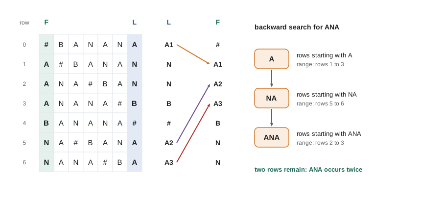
The key property is last-to-first (LF) mapping: the \(i\)-th occurrence of a character in the last column corresponds to the \(i\)-th occurrence of the same character in the first column, because both orderings are determined by what follows the character. Using LF mapping, the original text can be reconstructed backward from the BWT alone. Paolo Ferragina and Giovanni Manzini showed in 2000 that the same property allows counting occurrences of a pattern by processing it from its last character to its first, maintaining a range of rows in the sorted matrix that begin with the pattern suffix seen so far. Each step needs only two pieces of information: \(C(c)\), the number of characters in the text smaller than \(c\), and \(\mathrm{Occ}(c, i)\), the number of occurrences of \(c\) in the first \(i\) positions of the BWT. Together with a sampled suffix array that converts matrix rows back to text positions, this is the FM-index.
Each character of the pattern narrows the range in constant time, so searching for a pattern of length \(m\) takes time proportional to \(m\), regardless of the genome's size. Occurrence counts are stored at checkpoints every so many positions and computed between them, and the suffix array is stored only for a sample of positions, so the whole index of the human genome fits in about 4 to 5 gigabytes.
# Build a BWT and FM-index for a small text and count/locate patterns by backward search.
def build(text):
    text += '#'
    sa = sorted(range(len(text)), key=lambda i: text[i:])        # suffix array (fine for small texts)
    bwt = ''.join(text[i - 1] for i in sa)
    alphabet = sorted(set(text))
    C, total = {}, 0
    for ch in alphabet:
        C[ch] = total
        total += text.count(ch)
    occ = {ch: [0] for ch in alphabet}                              # occ[ch][i] = count in bwt[:i]
    for b in bwt:
        for ch in alphabet:
            occ[ch].append(occ[ch][-1] + (b == ch))
    return sa, bwt, C, occ

def search(pattern, index):
    sa, bwt, C, occ = index
    lo, hi = 0, len(bwt)
    for ch in reversed(pattern):
        if ch not in C:
            return []
        lo, hi = C[ch] + occ[ch][lo], C[ch] + occ[ch][hi]
        if lo >= hi:
            return []
    return sorted(sa[lo:hi])

print('BWT of BANANA:', build('BANANA')[1])
ref = 'ACGTTGCAACGTAGCTAGGCTAACGTTGCATCGATCGTAACGTTGCA'
idx = build(ref)
for p in ['ACGTTGCA', 'GCTAG', 'CGATCG', 'TTTT']:
    hits = search(p, idx)
print(f"{p:9s} occurrences {len(hits)} at positions {hits}")BWT of BANANA: ANNB#AA ACGTTGCA occurrences 3 at positions [0, 22, 39] GCTAG occurrences 1 at positions [13] CGATCG occurrences 1 at positions [31] TTTT occurrences 0 at positions []
Seed, chain and extend
For short reads, BWA-MEM finds maximal exact matches between the read and the reference using the FM-index, keeps seeds long enough to be informative, groups nearby seeds that are consistent with one location, and extends the best groups with Smith–Waterman-style alignment, allowing mismatches and gaps. Because seeds are exact, a read with an error every 20 bases still contains several error-free seeds of 19 bases or more. Bowtie 2 uses a similar strategy with multiple seed offsets.
Long reads need a different balance. A 20 kb nanopore read with one error every 100 bases contains many seeds, and full dynamic programming over 20 kb is expensive. Heng Li's minimap2, released in 2018 and now the standard long-read mapper, indexes minimizers of the reference in a hash table, finds minimizer matches between the read and the reference, and chains them: it finds a set of matches that are collinear (increasing in both read and reference position) with consistent spacing, by a dynamic programming over anchors rather than bases. Only the gaps between chained anchors are aligned base by base. Chaining also lets minimap2 split a read that spans a structural variant into separate alignments, which is how long reads reveal large deletions, inversions and translocations.
# Toy seed-and-extend mapper: hash 12-mers of a reference with a duplicated segment, map reads with errors.
import random
random.seed(406)
seg = ''.join(random.choice('ACGT') for _ in range(300))
ref = ''.join(random.choice('ACGT') for _ in range(2000)) + seg + ''.join(random.choice('ACGT') for _ in range(1500)) + seg + ''.join(random.choice('ACGT') for _ in range(1200))
k = 12
index = {}
for i in range(len(ref) - k + 1):
    index.setdefault(ref[i:i + k], []).append(i)

def mismatches(a, b):
    return sum(x != y for x, y in zip(a, b))

def map_read(read):
    votes = {}
    for off in range(0, len(read) - k + 1, 4):                  # seeds every 4 bases
        for pos in index.get(read[off:off + k], []):
            start = pos - off
            votes[start] = votes.get(start, 0) + 1
    scored = sorted(((mismatches(read, ref[s:s + len(read)]), s) for s in votes if 0 <= s <= len(ref) - len(read)))
    if not scored:
        return None, None, 0
    best = scored[0]
    second = scored[1][0] if len(scored) > 1 else len(read)
    mapq = 0 if second == best[0] else min(60, 10 * (second - best[0]))
    return best[1], best[0], mapq

def make_read(start, n=100, err=0.02):
    r = list(ref[start:start + n])
    for i in range(n):
        if random.random() < err:
            r[i] = random.choice([b for b in 'ACGT' if b != r[i]])
    return ''.join(r)

for true_start in (500, 2100, 3000, 3900):
    pos, mm, mapq = map_read(make_read(true_start))
print(f"true start {true_start:4d}: mapped to {pos}, mismatches {mm}, MAPQ {mapq}")true start 500: mapped to 500, mismatches 1, MAPQ 60 true start 2100: mapped to 2100, mismatches 1, MAPQ 0 true start 3000: mapped to 3000, mismatches 0, MAPQ 60 true start 3900: mapped to 2100, mismatches 3, MAPQ 0
Reads from unique sequence map confidently. Reads from inside the duplicated segment match two places equally well, so the mapper cannot tell which copy they came from: it picks one, often at random, and reports a mapping quality of zero. Real mappers compute mapping quality (MAPQ) as a Phred-scaled estimate of the probability that the reported position is wrong, based on the difference between the best and second-best alignment scores; MAPQ 0 means the read is equally likely to belong elsewhere, and MAPQ 60 is BWA's maximum. Variant callers usually ignore reads below a MAPQ threshold, which means that variants in segmental duplications and other repeats are hard to detect with short reads. The fraction of a genome in which reads of a given length can be placed uniquely is its mappability.
The SAM format
Mapping results are written in the Sequence Alignment/Map (SAM) format, defined in 2009 alongside the samtools software, or in its compressed binary equivalent BAM, or in CRAM, which stores reads as differences from the reference. A SAM file has header lines beginning with @, describing the reference sequences and the programs used, followed by one tab-separated line per alignment with eleven mandatory fields.
| Field | Name | Meaning |
|---|---|---|
| 1 | QNAME | Read name |
| 2 | FLAG | Bitwise flags: paired (1), properly paired (2), unmapped (4), mate unmapped (8), reverse strand (16), mate reverse (32), first in pair (64), second in pair (128), secondary (256), failed QC (512), duplicate (1024), supplementary (2048) |
| 3 | RNAME | Reference sequence name, such as chr7 |
| 4 | POS | 1-based leftmost mapping position |
| 5 | MAPQ | Mapping quality, Phred-scaled |
| 6 | CIGAR | Alignment operations: M match or mismatch, I insertion, D deletion, N skipped region (intron), S soft clip, H hard clip, = match, X mismatch |
| 7 to 9 | RNEXT, PNEXT, TLEN | Mate reference, mate position, observed template length |
| 10 | SEQ | Read sequence (reverse-complemented if on the reverse strand) |
| 11 | QUAL | Phred+33 base qualities |
# Decode FLAG bits and CIGAR strings from invented SAM lines; compute the reference span of each alignment.
import re
sam = """r001\t99\tchr2\t10511\t60\t8M2I40M\t=\t10750\t289\tSEQ\tQUAL
r001\t147\tchr2\t10750\t60\t50M\t=\t10511\t-289\tSEQ\tQUAL
r002\t0\tchr2\t20044\t42\t5S30M3D15M\t*\t0\t0\tSEQ\tQUAL
r003\t16\tchr5\t88120\t0\t50M\t*\t0\t0\tSEQ\tQUAL
r004\t1024\tchr2\t10511\t60\t50M\t*\t0\t0\tSEQ\tQUAL
r005\t4\t*\t0\t0\t*\t*\t0\t0\tSEQ\tQUAL"""
BITS = {1: 'paired', 2: 'proper pair', 4: 'unmapped', 8: 'mate unmapped', 16: 'reverse', 32: 'mate reverse',
        64: 'first', 128: 'second', 256: 'secondary', 512: 'QC fail', 1024: 'duplicate', 2048: 'supplementary'}
for line in sam.splitlines():
    f = line.split('\t')
    flag, pos, mapq, cigar = int(f[1]), int(f[3]), int(f[4]), f[5]
    names = [n for b, n in BITS.items() if flag & b]
    ops = re.findall(r'(\d+)([MIDNSHP=X])', cigar)
    ref_span = sum(int(n) for n, op in ops if op in 'MDN=X')
    clipped = sum(int(n) for n, op in ops if op == 'S')
    end = pos + ref_span - 1 if ref_span else None
print(f"{f[0]} flag {flag:4d} [{', '.join(names)}] {f[2]}:{pos}-{end} MAPQ {mapq} soft-clipped {clipped}")r001 flag 99 [paired, proper pair, mate reverse, first] chr2:10511-10558 MAPQ 60 soft-clipped 0 r001 flag 147 [paired, proper pair, reverse, second] chr2:10750-10799 MAPQ 60 soft-clipped 0 r002 flag 0 [] chr2:20044-20091 MAPQ 42 soft-clipped 5 r003 flag 16 [reverse] chr5:88120-88169 MAPQ 0 soft-clipped 0 r004 flag 1024 [duplicate] chr2:10511-10560 MAPQ 60 soft-clipped 0 r005 flag 4 [unmapped] *:0-None MAPQ 0 soft-clipped 0
BAM files are usually sorted by position and indexed so that tools can retrieve the reads overlapping any region instantly, which is how genome browsers display reads. Duplicate marking flags PCR duplicates (flag 1024) so that variant callers can ignore them. Supplementary alignments (flag 2048) represent the parts of a chimeric read that map elsewhere, the signature of structural variants and fusion genes.
Reference choice and reference bias
Every mapping-based analysis depends on its reference. Reads carrying the reference allele at a heterozygous site align slightly better than reads carrying the alternative allele, so the alternative is under-counted, a subtle reference bias that grows in divergent regions and in populations poorly represented in the reference. Reads from sequence missing from the reference map elsewhere, creating false variants, or not at all. Moving from GRCh38 to the complete T2T-CHM13 reference reduces false variant calls in previously unresolved regions and adds many genes to analysis, although clinical pipelines adopt new references cautiously because annotations and databases must be lifted over. Pangenome graph references go further: tools such as vg and graph-aware versions of standard mappers align reads to a graph that includes common alternative alleles, reducing reference bias across populations.
Worked problem
Why are there no variant calls in this gene?
A clinical exome pipeline reports no variants and patchy coverage in a gene that has a nearly identical pseudogene elsewhere in the genome. Most reads in the gene have MAPQ 0. Explain and suggest solutions.
Show solution
- A pseudogene with nearly identical sequence makes reads from either copy match both locations equally well.
- The mapper assigns such reads MAPQ 0 and places them at random between the two copies.
- Variant callers filter out low-MAPQ reads, so the gene appears to have low usable coverage and variants are missed.
- Solutions: use long reads that extend into flanking unique sequence; use paired-end reads with longer inserts; apply specialized callers designed for such genes; or confirm with a gene-specific long-range PCR assay.
- Report the gene as a region of limited sensitivity rather than as having no variants.
Answer: Low mappability due to the pseudogene; use longer-range information or specific assays, and report the limitation.
Common mistakes
MistakeTreating MAPQ 0 reads as reliable evidence at their reported position.
InsteadMAPQ 0 means the read maps equally well elsewhere; filter or handle such reads specially.
MistakeReading POS in SAM as 0-based.
InsteadSAM positions are 1-based; BED intervals are 0-based, half-open, a common source of off-by-one errors.
MistakeAssuming a CIGAR of 100M means 100 matching bases.
InsteadM means aligned bases, which may be matches or mismatches; = and X distinguish them.
MistakeIgnoring reference bias in heterozygous allele counts.
InsteadReads with the alternative allele map slightly less well; graph references or allele-aware methods reduce the bias.
MistakeForgetting that reverse-strand reads are stored reverse-complemented.
InsteadSEQ is given on the reference strand; check flag 16 before interpreting read orientation.
Summary and key terms
- Mapping places reads on a reference using fast seed lookup followed by verification with dynamic programming.
- The Burrows–Wheeler transform and FM-index allow exact matching in time proportional to pattern length, using LF mapping, C and Occ tables and a sampled suffix array.
- Short-read mappers (BWA-MEM, Bowtie 2) extend exact-match seeds; minimap2 chains minimizer anchors for long reads and splits reads at structural variants.
- Mapping quality is a Phred-scaled probability that the position is wrong; repeats yield MAPQ 0 and low mappability.
- SAM, BAM and CRAM store alignments with FLAG, POS, MAPQ and CIGAR fields; sorted, indexed BAMs allow regional queries.
- Reference bias and missing sequence affect results; T2T and pangenome references reduce them.
- read mapping
- Finding the most likely reference location for each read.
- seed
- A short exact match used to find candidate alignment locations.
- Burrows–Wheeler transform
- A reversible permutation of a text, taken from the last column of its sorted rotations.
- FM-index
- A compressed index built from the BWT that supports fast pattern search.
- LF mapping
- The correspondence between occurrences of a character in the last and first columns of the BWT matrix.
- suffix array
- The sorted list of starting positions of all suffixes of a text.
- chaining
- Selecting collinear seed matches that support one alignment.
- mapping quality
- A Phred-scaled probability that a read is mapped to the wrong location.
- mappability
- The extent to which reads from a region can be uniquely placed.
- CIGAR string
- A compact description of alignment operations such as matches, insertions, deletions and clips.
- reference bias
- Systematic preference for reads carrying the reference allele.
Practice problems
Work each problem on paper first, then reveal the answer to check.
Compute the BWT of ACAACG#.
Show answer
The sorted rotations end in G, C, #, A, A, A and C, so the BWT is GC#AAAC.
Why does backward search take time proportional to the pattern length, not the genome length?
Show answer
Each pattern character updates the row range in constant time using C and Occ.
A read has FLAG 83. Decode it.
Show answer
83 = 64 + 16 + 2 + 1: paired, properly paired, reverse strand, first in pair.
A read aligned at POS 1000 has CIGAR 10S60M5D30M. What reference interval does it cover?
Show answer
60 + 5 + 30 = 95 bases: positions 1000 to 1094.
What does MAPQ 20 mean?
Show answer
A 1 in 100 estimated probability that the mapping position is wrong.
Why do long-read mappers chain anchors instead of aligning the whole read immediately?
Show answer
Chaining finds the consistent location cheaply; base-level alignment is needed only between anchors.
How do supplementary alignments reveal structural variants?
Show answer
Parts of a read mapping to different locations or orientations indicate a rearrangement joining them.
Give one benefit of mapping to a pangenome graph.
Show answer
Reads with common non-reference alleles align correctly, reducing reference bias.
Lesson quiz · 5 questions
Score 60% or more to complete this lesson.
Create a free account to save your progress, take quizzes and earn a certificate.