
BIOL-410 · Lesson 5 of 12 · 26 min
Pairwise alignment and database search
Comparing sequences is the most common operation in bioinformatics. Aligning a newly sequenced gene against a database suggests its function; aligning a read against a reference places it in the genome; aligning homologous genes from different species reveals which positions are conserved by selection. This lesson develops the dynamic programming algorithms that find optimal alignments, the scoring systems that define what optimal means, the statistics that tell whether a match is meaningful, and the heuristics, above all BLAST, that make searching enormous databases fast.
Similarity and homology
Two sequences are homologous if they descend from a common ancestor. Homology is a yes-or-no statement about history; it is inferred, never measured directly. Similarity, the fraction of identical or chemically similar positions in an alignment, is what we measure, and high similarity is evidence for homology. Saying that two proteins are '40 per cent homologous' is therefore a common error: they may be 40 per cent identical, which strongly suggests that they are homologous. Homologues that diverged after a speciation event are orthologues; those that diverged after a gene duplication are paralogues, a distinction lesson 10 develops.
For proteins, sequence identity above about 30 to 35 per cent over a long alignment almost always indicates homology and usually a similar three-dimensional structure; below about 20 to 25 per cent, the so-called twilight zone, chance alignments become common and more sensitive methods, such as profile searches or structure comparison, are needed. For DNA, with only four letters, two random sequences already match at 25 per cent of aligned positions, so nucleotide comparisons lose sensitivity quickly for distant relationships. This is why database searches for gene function are usually done at the protein level, translating DNA if necessary.
Scoring alignments
An alignment places two sequences in columns, possibly inserting gaps, written as dashes, to bring homologous positions into register. Its score is the sum of scores for aligned pairs plus penalties for gaps. For DNA, a simple scheme scores +1 for a match and −1 for a mismatch, or reflects that transitions (purine to purine, pyrimidine to pyrimidine) are commoner than transversions. For proteins, substitution matrices capture the fact that some amino acid replacements are far more common in evolution than others: leucine for isoleucine, both hydrophobic, is frequent, while tryptophan for glycine is rare.
Substitution matrices are log-odds scores. If \(q_{ab}\) is the frequency with which residues \(a\) and \(b\) are aligned in trusted alignments of related proteins, and \(p_a\), \(p_b\) are their background frequencies, then the score compares the probability of the pair under homology with its probability by chance:
A positive score means the pair occurs more often in related proteins than by chance. Margaret Dayhoff's PAM matrices (1978) were derived from closely related proteins and extrapolated to greater distances; Steven and Jorja Henikoff's BLOSUM matrices (1992) were counted directly from conserved blocks of aligned sequences clustered at different identity levels. BLOSUM62, from blocks clustered at 62 per cent identity, is the default in protein BLAST; BLOSUM45 suits more distant relationships and BLOSUM80 closer ones. Because scores are log-odds, summing them over an alignment corresponds to multiplying probabilities, which gives alignment scores a statistical meaning.
# Derive log-odds scores (in half-bits, like BLOSUM) from a small invented set of aligned residue pairs.
import math
from collections import Counter
aligned = ["LIVLIVLLIIFLLIVMLLIV", "IVVLIIIMLVFLIVIMLIVV",   # invented trusted alignment, row 1 vs row 2
           "KRKKRDEDEKRRKEDDEKRK", "RKKRRDEEDKKRRDEEDRKK"]
pairs = Counter()
for a_row, b_row in ((aligned[0], aligned[1]), (aligned[2], aligned[3])):
    for a, b in zip(a_row, b_row):
        pairs[tuple(sorted((a, b)))] += 1
total = sum(pairs.values())
res = Counter()
for (a, b), n in pairs.items():
    res[a] += n
    res[b] += n
p = {r: n / (2 * total) for r, n in res.items()}
def score(a, b):
    key = tuple(sorted((a, b)))
    q = pairs.get(key, 0.5) / total            # pseudocount for unseen pairs
    expected = p[a] * p[b] * (1 if a == b else 2)
    return round(2 * math.log2(q / expected))
for a, b in [('L', 'L'), ('L', 'I'), ('I', 'V'), ('K', 'R'), ('D', 'E'), ('L', 'K'), ('V', 'D')]:
print(f"s({a},{b}) = {score(a, b):+d}")s(L,L) = +3 s(L,I) = +3 s(I,V) = +4 s(K,R) = +4 s(D,E) = +6 s(L,K) = -4 s(V,D) = -2
Even this tiny invented data set reproduces the qualitative pattern of real matrices: identities and conservative substitutions within the hydrophobic group or within the charged group score positively, and substitutions between groups score negatively. Real matrices are built from many thousands of aligned blocks.
Gaps represent insertions or deletions (indels). A linear gap penalty charges a constant amount per gap position, but biologically a single indel event often inserts or deletes several residues at once, so it should cost more to open a gap than to extend it. Affine gap penalties charge \(o + e(\ell - 1)\) for a gap of length \(\ell\), with opening penalty \(o\) larger than extension penalty \(e\); BLASTP's defaults with BLOSUM62 are 11 to open and 1 to extend. Osamu Gotoh showed in 1982 that affine gaps can be handled by dynamic programming with three matrices instead of one, at the same quadratic cost.
Global alignment: Needleman–Wunsch
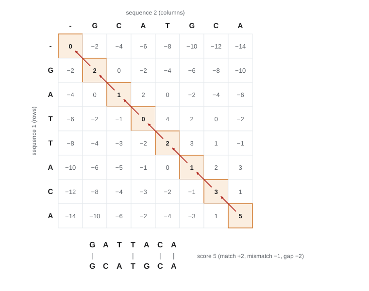
In 1970 Saul Needleman and Christian Wunsch introduced dynamic programming to sequence comparison. To align sequences \(x\) of length \(m\) and \(y\) of length \(n\) end to end, fill a matrix \(F\) in which \(F(i, j)\) is the best score of aligning the first \(i\) characters of \(x\) with the first \(j\) of \(y\). Each cell depends only on three neighbours: the best alignment ending at \((i, j)\) either aligns \(x_i\) with \(y_j\), or aligns \(x_i\) to a gap, or aligns \(y_j\) to a gap. With a linear gap penalty \(d\):
The first row and column hold the costs of leading gaps. Once the matrix is filled, the optimal score is in the bottom-right cell, and tracing back the choices that produced each cell recovers the alignment. The time and memory are proportional to \(mn\), which is fine for genes but impractical for whole chromosomes, where linear-memory variants and heuristics are used.
# Needleman-Wunsch global alignment and Smith-Waterman local alignment with traceback.
def align(x, y, match=2, mismatch=-1, gap=-2, local=False):
    m, n = len(x), len(y)
    F = [[0] * (n + 1) for _ in range(m + 1)]
    if not local:
        for i in range(1, m + 1): F[i][0] = i * gap
        for j in range(1, n + 1): F[0][j] = j * gap
    best, best_cell = -10**9, (m, n)
    for i in range(1, m + 1):
        for j in range(1, n + 1):
            s = match if x[i - 1] == y[j - 1] else mismatch
            F[i][j] = max(F[i - 1][j - 1] + s, F[i - 1][j] + gap, F[i][j - 1] + gap, 0 if local else -10**9)
            if local and F[i][j] > best:
                best, best_cell = F[i][j], (i, j)
    i, j = best_cell if local else (m, n)
    score = F[i][j]
    ax, ay = [], []
    while i > 0 or j > 0:
        if local and F[i][j] == 0:
            break
        s = match if i and j and x[i - 1] == y[j - 1] else mismatch
        if i and j and F[i][j] == F[i - 1][j - 1] + s:
            ax.append(x[i - 1]); ay.append(y[j - 1]); i -= 1; j -= 1
        elif i and F[i][j] == F[i - 1][j] + gap:
            ax.append(x[i - 1]); ay.append('-'); i -= 1
        else:
            ax.append('-'); ay.append(y[j - 1]); j -= 1
    return score, ''.join(reversed(ax)), ''.join(reversed(ay))

for kind, x, y, loc in [('global', 'GATTACA', 'GCATGCA', False),
                          ('global', 'TTGCCATGACCTGAAA', 'GCCATGTCCTG', False),
                          ('local ', 'TTGCCATGACCTGAAA', 'GCCATGTCCTG', True)]:
    sc, a, b = align(x, y, local=loc)
    print(f"{kind} score {sc:3d}")
    print('   ', a)
    print('   ', ''.join('|' if p == q else ' ' for p, q in zip(a, b)))
print(' ', b)global score 5
GATTACA
| | ||
GCATGCA
global score 9
TTGCCATGACCTGAAA
|||||| ||||
--GCCATGTCCTG---
local score 19
GCCATGACCTG
|||||| ||||
GCCATGTCCTGLocal alignment: Smith–Waterman
Often only part of two sequences is related: a shared protein domain in otherwise different proteins, or a gene within a long genomic region. Temple Smith and Michael Waterman's 1981 modification finds the best local alignment by adding a fourth option, zero, to the recurrence, so that an alignment can start fresh anywhere rather than carrying forward a negative score; the best local alignment ends at the highest cell anywhere in the matrix, and traceback stops when a zero is reached. In the example, global alignment of the two sequences of different length is forced to pay for end gaps, while the local alignment picks out the shared core. Semi-global alignment, which does not penalize gaps at the ends of one sequence, is what read mapping needs: the whole read should align, but only to part of the reference.
Alignment statistics
Any two sequences have a best local alignment, so a score alone does not show that they are related. Samuel Karlin and Stephen Altschul showed in 1990 that for local alignments without gaps the maximum scores of random sequences follow an extreme value distribution, and the expected number of chance alignments with score at least \(S\) when comparing a query of length \(m\) with a database of total length \(n\) is
where \(K\) and \(\lambda\) depend on the scoring system and residue frequencies (and are estimated empirically for gapped alignments). The E-value is the number of hits this good expected by chance in a search of this size; an E-value of 0.001 means one such chance hit per thousand searches. It grows with database size, so the same alignment is less significant in a bigger database. Bit scores normalize raw scores, \(S' = (\lambda S - \ln K)/\ln 2\), so that \(E = mn\,2^{-S'}\), making scores comparable across scoring systems.
# E-values for a hit of a given bit score against databases of different sizes.
query_len = 350                       # amino acids
for db_name, db_len in [('curated database', 2.0e8), ('large protein database', 1.0e11)]:
    for bits in (30, 40, 50, 80):
        e = query_len * db_len * 2 ** (-bits)
print(f"{db_name:22s} bit score {bits:3d}: E = {e:.2e}")curated database bit score 30: E = 6.52e+01 curated database bit score 40: E = 6.37e-02 curated database bit score 50: E = 6.22e-05 curated database bit score 80: E = 5.79e-14 large protein database bit score 30: E = 3.26e+04 large protein database bit score 40: E = 3.18e+01 large protein database bit score 50: E = 3.11e-02 large protein database bit score 80: E = 2.90e-11
BLAST and fast database search
Smith–Waterman is too slow to compare a query against hundreds of millions of sequences, so database search uses heuristics. BLAST (Basic Local Alignment Search Tool), published by Stephen Altschul, David Lipman and colleagues at NCBI in 1990, finds short word matches, called seeds (by default 3 residues for proteins and 11 or more bases for DNA, with similar words scoring above a threshold also counted for proteins), extends them without gaps into high-scoring segment pairs, and then performs gapped extension only around promising hits. It may miss some alignments that Smith–Waterman would find, but it is orders of magnitude faster, and its E-values make results interpretable. BLAST is one of the most cited scientific papers ever published.
| Program | Query | Database | Typical use |
|---|---|---|---|
| blastn | Nucleotide | Nucleotide | Identify a DNA sequence, find close relatives |
| blastp | Protein | Protein | Find homologues and infer function |
| blastx | Nucleotide, translated in 6 frames | Protein | Find protein-coding regions in DNA or reads |
| tblastn | Protein | Nucleotide, translated | Find unannotated genes for a protein in genomes |
| tblastx | Translated nucleotide | Translated nucleotide | Distant comparisons of DNA (slow) |
Faster tools now handle the scale of modern data. DIAMOND searches protein databases thousands of times faster than BLASTX with similar sensitivity, using spaced seeds and reduced alphabets, and MMseqs2 clusters and searches billions of sequences. For distant homology, profile methods are more sensitive than pairwise ones: PSI-BLAST iteratively builds a position-specific scoring matrix from its own hits, and profile hidden Markov models, used by HMMER with the Pfam database of protein families, capture position-specific conservation and gap preferences (lesson 8).
Multiple sequence alignment
Aligning many sequences at once reveals conserved positions, motifs and the input for phylogenetic trees (BIOL-321 and lesson 10). Optimal multiple alignment by dynamic programming is exponential in the number of sequences, so tools use progressive alignment: compute pairwise distances, build a guide tree, and align sequences and groups of sequences in the order given by the tree, as in Clustal Omega; MUSCLE and MAFFT add iterative refinement. Progressive alignment is greedy, and errors made early, especially gaps placed in the wrong column, propagate. Alignment uncertainty can affect downstream inferences, so analysts inspect alignments visually and sometimes remove poorly aligned columns before building trees.
Worked problem
Interpreting a BLAST result
A 420-amino-acid protein predicted from an invented soil bacterium gives a best BLASTP hit with 28 per cent identity over 390 residues, bit score 112, E-value 3e−25, to a characterized glycoside hydrolase. The next hit, to an unrelated protein, has 34 per cent identity over 41 residues and E-value 2.1. What do you conclude?
Show solution
- Despite modest identity, the first hit covers most of the protein, and an E-value of 3e−25 means a match this good would occur by chance far less than once in the search.
- Long alignments in the 25 to 30 per cent identity range are usually homologous; the significance comes from the length.
- The second hit has higher identity but over only 41 residues; its E-value of 2.1 means two such hits are expected by chance, so it is not evidence of homology.
- Conclude that the protein is probably a homologue of glycoside hydrolases; confirm with a domain search against Pfam and check that catalytic residues are conserved before assigning a specific function.
Answer: The first hit indicates homology to glycoside hydrolases; the second is a chance match. Specific function requires further evidence.
Common mistakes
MistakeSaying two sequences are "40 per cent homologous".
InsteadHomology is all or nothing; report percentage identity or similarity, and infer homology from significance.
MistakeJudging hits by percentage identity alone.
InsteadShort alignments can have high identity by chance; use E-values or bit scores, which account for length and database size.
MistakeComparing E-values from searches of databases of different sizes as if equivalent.
InsteadE-values scale with database size; bit scores are comparable.
MistakeUsing global alignment to find a shared domain in otherwise unrelated proteins.
InsteadUse local alignment, which does not penalize unrelated flanking regions.
MistakeTransferring a precise function from a distant BLAST hit.
InsteadDistant homologues often have different specificities; check domains, active sites and experimental evidence.
Summary and key terms
- Homology is common ancestry, inferred from significant similarity; orthologues and paralogues differ in how they arose.
- Substitution matrices such as BLOSUM62 are log-odds scores; affine gaps charge more to open than to extend.
- Needleman–Wunsch finds optimal global alignments by dynamic programming in time proportional to mn; Smith–Waterman finds local alignments by adding a zero floor.
- E = Kmn e^−λS gives the expected number of chance hits; bit scores normalize raw scores across scoring systems.
- BLAST uses seeds, ungapped extension and selective gapped alignment to search large databases quickly; DIAMOND and MMseqs2 scale further.
- Progressive multiple alignment follows a guide tree; profile methods detect distant homology.
- homology
- Descent of sequences from a common ancestor.
- substitution matrix
- A table of log-odds scores for aligning each pair of residues.
- affine gap penalty
- A gap cost with a larger opening penalty and a smaller per-residue extension penalty.
- dynamic programming
- Solving a problem by combining optimal solutions to overlapping subproblems stored in a table.
- global alignment
- An alignment of two sequences over their entire lengths.
- local alignment
- An alignment of the most similar subsequences of two sequences.
- E-value
- The expected number of chance alignments scoring at least as well in a search of a given size.
- bit score
- A normalized alignment score independent of the scoring system.
- BLAST
- A heuristic tool that finds local alignments between a query and a database using seeds.
- progressive alignment
- Multiple alignment built by adding sequences in the order of a guide tree.
Practice problems
Work each problem on paper first, then reveal the answer to check.
Why do protein searches detect more distant homologues than DNA searches?
Show answer
Protein sequences have 20 letters and substitution matrices weight similar residues; DNA saturates quickly and random matches are common.
What does a positive log-odds score for a residue pair mean?
Show answer
The pair occurs more often in related proteins than expected by chance.
With gap opening 11 and extension 1, what is the cost of a 5-residue gap?
Show answer
11 + 4 x 1 = 15.
How does Smith–Waterman differ from Needleman–Wunsch in the recurrence and the traceback?
Show answer
It adds zero as an option and traces back from the highest cell until a zero is reached.
An alignment has E = 0.02 in a search of 10^8 residues. What would its E-value be in a database of 10^10 residues?
Show answer
About 2, a hundred times larger.
Which BLAST program would you use to find genes encoding a known protein in an unannotated genome?
Show answer
tblastn.
Why is progressive multiple alignment called greedy?
Show answer
Early pairwise decisions are fixed and not revisited, so their errors propagate.
What is the time complexity of Needleman–Wunsch for sequences of lengths m and n?
Show answer
Proportional to mn.
Lesson quiz · 5 questions
Score 60% or more to complete this lesson.
Create a free account to save your progress, take quizzes and earn a certificate.