
BIOL-410 · Lesson 11 of 12 · 26 min
Structural, functional and metagenomics
Sequencing is now used far beyond reading genomes. The same instruments measure where proteins bind DNA, which regions of chromatin are open, which cytosines are methylated, how chromosomes fold, which genes matter for a cell's survival, and which microbes live in a gut, a lake or a city's sewage. Meanwhile, computational methods predict protein structures from sequence with an accuracy that won the 2024 Nobel Prize in Chemistry. This lesson surveys these applications: structural bioinformatics, functional genomics assays, and metagenomics, including the wastewater surveillance that became part of public health during the COVID-19 pandemic.
From sequence to structure
Proteins act through their three-dimensional structures, and for decades determining a structure required X-ray crystallography, nuclear magnetic resonance or, increasingly, cryo-electron microscopy, months or years of work per protein. The Protein Data Bank, founded in 1971, now holds more than 200,000 experimentally determined structures, but that is a tiny fraction of the hundreds of millions of known protein sequences. Predicting structure from sequence, the protein folding problem, was a grand challenge, tracked since 1994 by the biennial Critical Assessment of Structure Prediction (CASP), in which groups predict structures that have been determined but not yet released.
At CASP14 in 2020, AlphaFold 2, developed by Google DeepMind, predicted many structures with accuracy comparable to experiment. It combines a deep neural network that reasons jointly over a multiple sequence alignment of the protein's homologues, whose co-varying positions hint at residues in contact, and over a representation of pairs of residues, with an explicit module that builds three-dimensional coordinates. Each residue receives a confidence score, the predicted local distance difference test (pLDDT), from 0 to 100; regions below about 50 are often intrinsically disordered rather than poorly predicted. In 2021 DeepMind and EMBL-EBI released predictions for the human proteome, and the AlphaFold Protein Structure Database now holds more than 200 million predicted structures, covering nearly all of UniProt. Other methods followed, including RoseTTAFold from David Baker's laboratory and ESMFold, which uses a protein language model instead of an alignment.
The 2024 Nobel Prize in Chemistry was awarded half to David Baker, for computational protein design, and half jointly to Demis Hassabis and John Jumper, for protein structure prediction. AlphaFold 3, published in 2024, extends prediction to complexes of proteins with nucleic acids, small molecules and ions. Predicted structures have transformed many projects, but they have limits: they show one static conformation, are less reliable for proteins with few homologues, and do not by themselves predict the effects of single mutations on stability or the dynamics of binding. They are hypotheses to test, not replacements for experiment.
Functional genomics: reading the regulatory genome
Most functional sequence in large genomes is not protein-coding (lesson 10), and sequencing-based assays map it. In chromatin immunoprecipitation followed by sequencing (ChIP-seq), proteins are cross-linked to DNA, the chromatin is fragmented, an antibody pulls down a chosen transcription factor or modified histone, and the attached DNA is sequenced. Reads pile up where the protein binds. Peak callers such as MACS compare read density with a control sample, input DNA without immunoprecipitation, to find regions with significantly more reads than expected, using a local Poisson model to account for background differences in chromatin and mappability. ATAC-seq uses a hyperactive transposase that preferentially inserts sequencing adapters into open, accessible chromatin, mapping regulatory regions genome-wide from small numbers of cells, including single cells.
# Toy peak calling: count ChIP and input reads in 200 bp windows and test for enrichment with a Poisson model.
import numpy as np
from scipy import stats
rng = np.random.default_rng(11)
L, w = 100_000, 200
n_win = L // w
bg = rng.gamma(4, 0.25, n_win)                       # background varies along the region
input_counts = rng.poisson(bg * 10)
chip_rate = bg * 10.0
peaks_true = [57, 140, 141, 333]                     # windows with real binding
for p in peaks_true:
    chip_rate[p] *= 8
chip_counts = rng.poisson(chip_rate)
scale = chip_counts.sum() / input_counts.sum()
lam = np.maximum(input_counts * scale, chip_counts.mean() * 0.5)    # local expectation with a floor
pvals = stats.poisson.sf(chip_counts - 1, lam)
qcut = 1e-6
called = np.where(pvals < qcut)[0]
print('windows tested:', n_win, ' threshold p <', qcut)
for i in called:
    print(f"window {i:3d} ({i * w:6d}-{(i + 1) * w:6d}): ChIP {chip_counts[i]:3d}, expected {lam[i]:5.1f}, p = {pvals[i]:.1e}")
print('true binding windows:', peaks_true)windows tested: 500 threshold p < 1e-06 window 57 ( 11400- 11600): ChIP 60, expected 5.5, p = 2.1e-40 window 140 ( 28000- 28200): ChIP 82, expected 8.6, p = 2.0e-50 window 141 ( 28200- 28400): ChIP 91, expected 16.1, p = 7.5e-38 window 333 ( 66600- 66800): ChIP 139, expected 15.1, p = 1.9e-82 true binding windows: [57, 140, 141, 333]
All four planted binding windows are called and no others pass the strict threshold, even though background coverage varies severalfold along the region, because each window is judged against its own local expectation from the input. Two adjacent windows form one broader peak, as real peaks often span several hundred bases. Testing 500 windows at p below one in a million keeps the expected number of false calls far below one; genome-wide, peak callers report false discovery rates instead.
DNA methylation, chiefly 5-methylcytosine at CG dinucleotides in vertebrates, is measured by bisulfite sequencing, which converts unmethylated cytosines to uracil (read as thymine) while methylated ones remain cytosine, so methylation is read as C versus T at each CG; enzymatic conversion methods do the same with less DNA damage, and long-read platforms detect methylation directly (lesson 2). Hi-C (lesson 4) maps the three-dimensional folding of chromosomes, revealing compartments and topologically associating domains within which regulatory contacts are concentrated. The ENCODE project, begun in 2003, and its successors have applied these assays systematically across human and mouse cell types, producing catalogues of candidate regulatory elements.
Functional genomics also asks which genes are needed. In a pooled CRISPR screen, a library of guide RNAs targeting every gene, typically four or more guides per gene, is delivered to a large population of cells so that each cell receives one guide, and the cells are grown under a selection, such as a drug. Guides are sequenced before and after selection; guides targeting genes whose loss confers resistance become enriched, and those targeting genes essential under the condition are depleted. Counting guides is an RNA-seq-like count problem, and tools such as MAGeCK combine guide-level evidence into gene-level scores.
# Gene-level scores from an invented pooled CRISPR screen: four guides per gene, counts before and after drug selection.
import numpy as np
rng = np.random.default_rng(5)
genes = ['GENE1', 'GENE2', 'GENE3', 'GENE4', 'GENE5', 'ESS1', 'RES1', 'CTRL']
effect = {'ESS1': -2.5, 'RES1': 3.0}                   # log2 effect of knockout under selection
before, after, names = [], [], []
for g in genes:
    for k in range(4):
        b = rng.poisson(500)
        lfc = effect.get(g, 0) + rng.normal(0, 0.3) + (rng.normal(0, 1.2) if k == 3 and g == 'GENE2' else 0)
        before.append(b); after.append(rng.poisson(b * 2 ** lfc)); names.append(g)
before, after = np.array(before, float), np.array(after, float)
lfc = np.log2((after / after.sum() * 1e6 + 1) / (before / before.sum() * 1e6 + 1))
lfc -= np.median(lfc)
print(f"{'gene':6s} guide log2 fold changes            median")
for g in genes:
    v = lfc[[i for i, n in enumerate(names) if n == g]]
print(f"{g:6s} {' '.join(f'{x:+5.2f}' for x in v)} {np.median(v):+5.2f}")gene guide log2 fold changes median GENE1 -0.06 -0.14 +0.20 -0.07 -0.06 GENE2 +0.26 +0.05 -0.29 +1.18 +0.15 GENE3 +0.07 +0.42 +0.27 -0.09 +0.17 GENE4 +0.11 +0.13 -0.00 -0.14 +0.06 GENE5 -0.05 -0.57 +0.00 +0.09 -0.02 ESS1 -2.36 -2.43 -2.65 -2.35 -2.40 RES1 +3.15 +3.27 +3.52 +2.78 +3.21 CTRL -0.09 +0.03 -0.17 -0.50 -0.13
Using the median of several guides protects against a single guide with an off-target or inefficient effect, as shown by the one aberrant guide for GENE2: the median of that gene stays near zero. The essential gene's guides are consistently depleted and the resistance gene's guides consistently enriched.
Metagenomics: sequencing communities
Most microbes have never been grown in the laboratory, so sequencing DNA directly from environmental or clinical samples, metagenomics, has revealed a vast diversity of life, including whole new phyla of bacteria and archaea. There are two main approaches. Amplicon sequencing amplifies a marker gene, usually one or more variable regions of the 16S ribosomal RNA gene for bacteria and archaea, or the internal transcribed spacer for fungi, and sequences the products. It is cheap and sensitive, but resolves taxa only to genus level in many cases, is biased by primer choice and by differences in 16S copy number between species, and reveals nothing directly about functions. Modern pipelines such as DADA2 infer exact amplicon sequence variants (ASVs), correcting sequencing errors statistically, rather than clustering reads into operational taxonomic units at 97 per cent identity as older methods did.
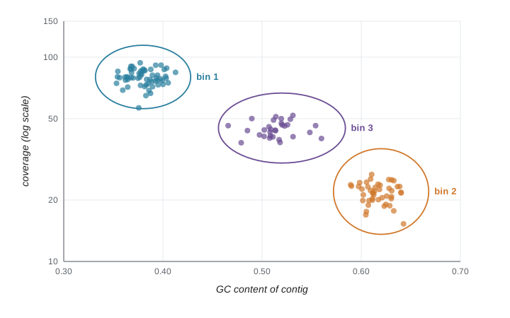
Shotgun metagenomics sequences all DNA in the sample. Reads can be classified taxonomically by matching k-mers or marker genes against reference databases (Kraken2, MetaPhlAn), profiled for functions such as antibiotic resistance genes or metabolic pathways, and assembled into contigs. Contigs from the same genome share sequence composition (GC content, tetranucleotide frequencies) and, across samples, a similar pattern of coverage, so they can be grouped, or binned, into metagenome-assembled genomes (MAGs). Bin quality is estimated by the completeness and contamination of a set of single-copy marker genes, analogous to BUSCO (lesson 4); standards define high-quality MAGs as more than 90 per cent complete with less than 5 per cent contamination.
# Bin invented metagenomic contigs from two genomes by GC content and coverage with k-means.
import numpy as np
rng = np.random.default_rng(21)
n1, n2, n3 = 60, 45, 30
gc = np.concatenate([rng.normal(0.38, 0.015, n1), rng.normal(0.62, 0.015, n2), rng.normal(0.52, 0.02, n3)])
cov = np.concatenate([rng.normal(80, 8, n1), rng.normal(22, 3, n2), rng.normal(45, 5, n3)])
truth = np.repeat([0, 1, 2], [n1, n2, n3])
X = np.column_stack([(gc - gc.mean()) / gc.std(), (np.log(cov) - np.log(cov).mean()) / np.log(cov).std()])
best = None
for restart in range(10):
    c = X[rng.choice(len(X), 3, replace=False)]
    for _ in range(30):
        a = np.argmin(((X[:, None] - c[None]) ** 2).sum(-1), axis=1)
        c = np.array([X[a == j].mean(0) if np.any(a == j) else c[j] for j in range(3)])
    inertia = ((X - c[a]) ** 2).sum()
    if best is None or inertia < best[0]:
        best = (inertia, a)
a = best[1]
for j in range(3):
    m = a == j
    print(f"bin {j}: {m.sum():3d} contigs, mean GC {gc[m].mean():.2f}, mean coverage {cov[m].mean():5.1f}, "
f"true genomes {np.bincount(truth[m], minlength=3)}")bin 0: 45 contigs, mean GC 0.62, mean coverage 21.2, true genomes [ 0 45 0] bin 1: 60 contigs, mean GC 0.38, mean coverage 79.3, true genomes [60 0 0] bin 2: 30 contigs, mean GC 0.52, mean coverage 44.5, true genomes [ 0 0 30]
Metagenomic data are compositional: sequencing yields proportions, not absolute abundances, so an increase in one taxon necessarily lowers the proportions of others even if they did not change, the same composition problem met in RNA-seq. Diversity measures borrowed from ecology (BIOL-367) summarize communities: alpha diversity, such as the Shannon index, within a sample, and beta diversity, such as the Bray–Curtis dissimilarity, between samples. Contamination is a serious concern for low-biomass samples, where reagent DNA can dominate, so negative controls are essential.
Pathogen genomics and wastewater surveillance
Genomics now underpins public health microbiology (BIOL-330). Whole-genome sequencing of foodborne bacteria such as Salmonella and Listeria lets laboratories link cases separated in time and space by small numbers of single-nucleotide differences between isolates, defining outbreaks that traditional typing missed; national networks share sequences in real time. During the COVID-19 pandemic, genomic surveillance tracked SARS-CoV-2 lineages and identified variants of concern, and sequencing millions of viral genomes made it the most sequenced pathogen in history.
Wastewater surveillance measures pathogens in sewage, which pools material from thousands to millions of people regardless of whether they seek testing. Quantitative PCR measures viral RNA concentrations, normalized to flow or to human fecal markers, and sequencing identifies variant mixtures. Programs established for SARS-CoV-2 have expanded to influenza, respiratory syncytial virus, mpox, measles and antimicrobial resistance genes. Wastewater data are population-level and anonymous by design, but small sewersheds, such as a single building, raise privacy questions that programs address with minimum population thresholds.
In Canada, the Public Health Agency of Canada's National Microbiology Laboratory in Winnipeg coordinates a national wastewater surveillance program with provinces, municipalities and universities, and publishes trends for SARS-CoV-2, influenza and respiratory syncytial virus, among other targets. Ottawa was an early adopter, through a partnership of the University of Ottawa, the Children's Hospital of Eastern Ontario and Ottawa Public Health, and provincial programs operate in several provinces. The National Microbiology Laboratory also coordinates national pathogen genomics, including the Canadian COVID-19 Genomics Network (CanCOGeN), funded through Genome Canada, which sequenced hundreds of thousands of SARS-CoV-2 genomes.
| Approach | What is sequenced | Main outputs | Key caveats |
|---|---|---|---|
| 16S amplicon | A variable region of the 16S rRNA gene | Taxonomic composition (often to genus) | Primer bias, copy-number variation, no direct functions |
| Shotgun metagenomics | All DNA in the sample | Taxa, genes, pathways, MAGs | Host DNA, database gaps, cost |
| Metatranscriptomics | Community RNA | Active functions | RNA instability, rRNA removal |
| Wastewater qPCR and sequencing | Nucleic acids in sewage | Population-level pathogen trends and variants | Dilution, normalization, privacy in small sewersheds |
| Isolate whole-genome sequencing | Genomes of cultured pathogens | Outbreak linkage, resistance prediction | Requires culture; SNP thresholds context-dependent |
Worked problem
Interpreting an outbreak SNP distance
Listeria isolates from five patients in two provinces or states over six months differ by 0 to 4 single-nucleotide differences in their core genomes. An isolate from a cheese plant differs from them by 2 to 5, while unrelated isolates differ by more than 100. What can be concluded?
Show solution
- Differences of 0 to 4 SNPs among patient isolates indicate very close relatedness, consistent with a common source; unrelated isolates differ by hundreds.
- The plant isolate falls within the same small range, strongly suggesting it is the source or shares a source with the cases.
- Genomic data alone do not prove the route of transmission; epidemiological evidence (what patients ate, distribution records) must agree.
- SNP thresholds are not universal: they depend on the organism, its mutation rate and how long a contamination has persisted in a facility.
- Act on the combined evidence: genomic linkage plus epidemiology justifies investigation and possible recall at the plant.
Answer: The isolates form a tight genomic cluster with the plant isolate, supporting a common source, to be confirmed with epidemiological evidence.
Common mistakes
MistakeTreating a predicted protein structure as experimentally determined.
InsteadCheck confidence scores such as pLDDT and validate key conclusions experimentally.
MistakeCalling ChIP-seq peaks without an input control.
InsteadBackground varies along the genome; compare with input to avoid false peaks in open or high-copy regions.
MistakeInterpreting 16S relative abundance changes as absolute changes.
InsteadData are compositional; an increase in one taxon lowers others’ proportions.
MistakeAccepting low-quality bins as genomes.
InsteadReport completeness and contamination; high-quality MAGs exceed 90 per cent completeness with under 5 per cent contamination.
MistakeUsing a fixed SNP threshold to define outbreaks for every pathogen.
InsteadThresholds depend on organism, mutation rate and epidemiological context.
Summary and key terms
- AlphaFold 2 (2020) predicts protein structures with near-experimental accuracy; pLDDT expresses confidence, and over 200 million predictions are public.
- The 2024 Nobel Prize in Chemistry recognized Baker for protein design and Hassabis and Jumper for structure prediction; AlphaFold 3 models complexes.
- ChIP-seq, ATAC-seq, bisulfite sequencing and Hi-C map protein binding, accessibility, methylation and 3D folding; peaks are called relative to controls.
- Pooled CRISPR screens count guides before and after selection and combine guides into gene-level scores.
- 16S amplicon sequencing profiles taxa; shotgun metagenomics profiles taxa and functions and yields MAGs binned by composition and coverage.
- Pathogen genomics links outbreak cases, and wastewater surveillance tracks pathogens at the population level.
- pLDDT
- A per-residue confidence score from 0 to 100 for predicted protein structures.
- ChIP-seq
- Sequencing of DNA bound by an immunoprecipitated protein to map binding sites.
- peak calling
- Identifying genomic regions with significantly more reads than expected from a control.
- ATAC-seq
- A transposase-based assay that maps accessible chromatin.
- bisulfite sequencing
- Sequencing after conversion of unmethylated cytosines to uracil, to measure methylation.
- pooled CRISPR screen
- An experiment in which a library of guide RNAs is introduced into cells and guide abundance is tracked after selection.
- amplicon sequence variant
- An exact sequence inferred from amplicon reads after error correction.
- metagenome-assembled genome
- A genome reconstructed by binning contigs from a metagenome.
- compositional data
- Data that represent proportions of a whole, so components are not independent.
- wastewater surveillance
- Monitoring of pathogens or other markers in sewage to track community health.
Practice problems
Work each problem on paper first, then reveal the answer to check.
What does a pLDDT below 50 often indicate?
Show answer
An intrinsically disordered region rather than a folded structure.
Why is an input control used in ChIP-seq?
Show answer
To model background read density, which varies with chromatin, copy number and mappability.
In bisulfite sequencing, how does an unmethylated CG appear in reads?
Show answer
As TG (the C reads as T); methylated CG remains CG.
Why are several guides per gene used in CRISPR screens?
Show answer
To guard against off-target or inefficient guides; gene scores combine them robustly.
Give two limitations of 16S amplicon sequencing.
Show answer
Limited taxonomic resolution and primer or copy-number bias; it does not directly reveal functions.
What two kinds of information are used to bin contigs into MAGs?
Show answer
Sequence composition (GC, k-mer frequencies) and coverage across samples.
Why is metagenomic abundance data called compositional?
Show answer
Reads give proportions summing to a fixed total, not absolute abundances.
Why do wastewater programs set minimum population sizes for sewersheds?
Show answer
To protect privacy, since small sewersheds could reveal information about identifiable people.
Lesson quiz · 5 questions
Score 60% or more to complete this lesson.
Create a free account to save your progress, take quizzes and earn a certificate.