Optimization and generalization

In machine learning, optimization is a means, not an end. The goal is a model that performs well on new data, and the training loss is only a proxy for that. Remarkably, the choice of optimizer, step size, batch size, initialization and stopping time affects not only how fast the training loss falls but which solution is found, and different solutions with the same training loss can generalize very differently. This lesson examines that connection: explicit regularization, early stopping as a form of regularization, the implicit bias of gradient methods toward particular solutions, the role of step size and noise in finding flat regions of the loss, and methods such as sharpness-aware minimization that exploit these ideas.

Training loss, test loss and the gap

The empirical risk \(\hat{R}(w) = \frac{1}{n}\sum_i \ell(w; x_i, y_i)\) is what we minimize; the population risk \(R(w) = \mathbb{E}[\ell(w; x, y)]\) is what we care about. Their difference, the generalization gap, is small when the model cannot fit noise too closely, which classical theory ties to the capacity of the model class relative to \(n\). Optimization interacts with this in two ways: methods can stop before fitting noise, and among the many minimizers of an over-parameterized model, methods choose some rather than others.

Explicit regularization

The most direct approach adds a penalty to the objective: \(\hat{R}(w) + \lambda\Omega(w)\). An L2 penalty (ridge, weight decay) shrinks weights toward zero; an L1 penalty (lasso) sets many to zero (Lessons 2 and 7). From the optimization viewpoint, L2 regularization also improves conditioning (Lesson 2), making the problem easier as well as better behaved statistically. Note that in adaptive optimizers, an L2 penalty added to the loss is not the same as weight decay applied directly to the weights; AdamW decouples them (Lesson 5).

Early stopping

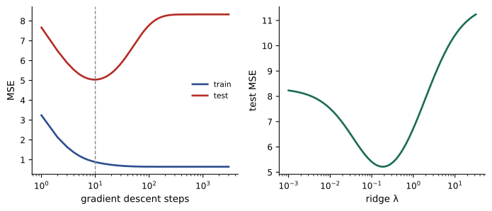
Gradient descent started from zero on a least-squares problem fits the directions of large curvature (the dominant patterns in the data) first, and the directions of small curvature (often noise) last. Stopping early therefore leaves the noise-dominated directions under-fitted, much as ridge regression shrinks them. For least squares the correspondence can be made precise: after \(k\) steps of size \(\eta\), each eigen-direction with curvature \(\sigma\) is fitted by a factor \(1 - (1 - \eta\sigma)^k\), while ridge with penalty \(\lambda\) fits it by \(\sigma/(\sigma + \lambda)\). Both act as filters that pass large-\(\sigma\) directions and suppress small ones, with \(\lambda \approx 1/(\eta k)\).

import numpy as np

rng = np.random.default_rng(7)
n, d = 60, 40
X = rng.normal(size=(n, d))
w_true = np.zeros(d); w_true[:5] = rng.normal(size=5) * 2
y = X @ w_true + rng.normal(0, 1.5, n)
Xt = rng.normal(size=(2000, d)); yt = Xt @ w_true + rng.normal(0, 1.5, 2000)

def test_mse(w):
    return np.mean((Xt @ w - yt) ** 2)

# Gradient descent on unregularized least squares, tracking test error over time
L = np.linalg.eigvalsh(X.T @ X / n).max()
w = np.zeros(d)
best = (np.inf, 0)
for k in range(1, 3001):
    w -= (X.T @ (X @ w - y) / n) / L
    e = test_mse(w)
    best = min(best, (e, k))
    if k in (5, 20, 100, 500, 3000):
        print(f"GD step {k:5d}: train MSE {np.mean((X @ w - y) ** 2):6.2f}  test MSE {e:6.2f}  ||w|| {np.linalg.norm(w):5.2f}")
print(f"best test MSE {best[0]:.2f} at step {best[1]}  (early stopping)")

# Ridge regression over a range of penalties for comparison
for lam in (10.0, 1.0, 0.1, 0.0):
    wr = np.linalg.solve(X.T @ X / n + lam * np.eye(d), X.T @ y / n)
    print(f"ridge lambda {lam:5.1f}: test MSE {test_mse(wr):6.2f}  ||w|| {np.linalg.norm(wr):5.2f}")

GD step     5: train MSE   1.20  test MSE   5.32  ||w||  2.22
GD step    20: train MSE   0.74  test MSE   5.37  ||w||  2.87
GD step   100: train MSE   0.65  test MSE   7.79  ||w||  3.33
GD step   500: train MSE   0.65  test MSE   8.33  ||w||  3.39
GD step  3000: train MSE   0.65  test MSE   8.33  ||w||  3.39
best test MSE 5.04 at step 10  (early stopping)
ridge lambda  10.0: test MSE  10.42  ||w||  0.30
ridge lambda   1.0: test MSE   6.74  ||w||  1.36
ridge lambda   0.1: test MSE   5.41  ||w||  2.61
ridge lambda   0.0: test MSE   8.33  ||w||  3.39

Early stopping is used almost universally in training neural networks: a validation set is evaluated periodically, and the checkpoint with the best validation score is kept. It costs nothing extra and needs no choice of penalty, only a stopping rule.

Implicit bias

Modern networks often have far more parameters than training examples and can reach zero training loss in many ways. Which zero-loss solution an optimizer finds is its implicit bias, and it can be characterized in simple cases:

• For under-determined least squares, gradient descent started from zero converges to the minimum-norm solution that fits the data exactly, because its iterates stay in the row space of the data.
• For logistic regression on separable data, the weights grow without bound, but their direction converges (slowly, at a rate like \(1/\log t\)) to the maximum-margin separator, the same direction a hard-margin support vector machine finds.
• Adaptive methods and different parameterizations have different biases; for example, training a product of matrices biases toward low-rank solutions.

import numpy as np

rng = np.random.default_rng(8)
# Underdetermined least squares: more parameters than examples, infinitely many exact fits
n, d = 20, 100
X = rng.normal(size=(n, d))
y = rng.normal(size=n)
w_min = np.linalg.pinv(X) @ y                    # minimum-norm interpolating solution

for name, w0 in (("zero start", np.zeros(d)), ("random start", rng.normal(size=d))):
    w = w0.copy()
    L = np.linalg.eigvalsh(X @ X.T).max()
    for _ in range(5000):
        w -= X.T @ (X @ w - y) / L
    print(f"{name:12s}: train residual {np.linalg.norm(X @ w - y):.1e}, ||w|| {np.linalg.norm(w):.3f}, "
          f"distance to min-norm solution {np.linalg.norm(w - w_min):.3f}")
print(f"min-norm solution ||w|| {np.linalg.norm(w_min):.3f}")

# Separable logistic regression: GD drives ||w|| to infinity but its direction approaches the max-margin one
Xs = np.array([[2.0, 1.0], [1.0, 3.0], [-1.0, -2.0], [-2.0, -0.5]])
ys = np.array([1, 1, -1, -1])
w = np.zeros(2)
for k in range(1, 200001):
    m = ys * (Xs @ w)
    w += 0.5 * (Xs.T @ (ys / (1 + np.exp(m)))) / 4
    if k in (100, 10000, 200000):
        u = w / np.linalg.norm(w)
        print(f"step {k:6d}: ||w|| {np.linalg.norm(w):6.2f}, direction {np.round(u, 3)}, min margin {np.min(ys * (Xs @ u)):.3f}")
angles = np.linspace(0, 2 * np.pi, 200001)
U = np.stack([np.cos(angles), np.sin(angles)], axis=1)
margins = np.min((U @ Xs.T) * ys, axis=1)
best = U[np.argmax(margins)]
print(f"max-margin direction {np.round(best, 3)}, margin {margins.max():.3f}")

zero start  : train residual 5.8e-16, ||w|| 0.675, distance to min-norm solution 0.000
random start: train residual 3.3e-15, ||w|| 9.645, distance to min-norm solution 9.622
min-norm solution ||w|| 0.675
step    100: ||w||   2.55, direction [0.765 0.644], min margin 1.852
step  10000: ||w||   4.81, direction [0.798 0.603], min margin 1.897
step 200000: ||w||   6.32, direction [0.807 0.59 ], min margin 1.910
max-margin direction [0.832 0.555], margin 1.941

These results suggest one explanation of why over-parameterized models can generalize: among the many interpolating solutions, gradient methods prefer simple ones (small norm, large margin), which generalize well. It also shows that initialization matters: the random start found an interpolating solution with a much larger norm.

Step size, noise and flat minima

Lesson 1 showed that gradient descent with step \(\eta\) is stable at a minimum only if its curvature is below \(2/\eta\). A minimum sharper than that is unstable: the iterates oscillate and are thrown out. Larger step sizes therefore select flatter minima, and the noise in stochastic gradients (Lesson 3) adds a further push away from narrow regions.

import numpy as np

# A loss with a sharp minimum near x = -1 (curvature about 50) and a flat one near x = 2 (curvature about 2)
def f(x):
    return -np.log(np.exp(-25 * (x + 1) ** 2) + np.exp(-(x - 2) ** 2) + 1e-12)

def grad(x, h=1e-6):
    return (f(x + h) - f(x - h)) / (2 * h)

def curvature(x, h=1e-4):
    return (f(x + h) - 2 * f(x) + f(x - h)) / h ** 2

print(f"curvature at sharp minimum {curvature(-1.0):.1f}, at flat minimum {curvature(2.0):.1f}")
starts = np.linspace(-1.6, 0.4, 9)
for lr in (0.01, 0.1):
    ends = []
    for x in starts:
        for _ in range(3000):
            x = x - lr * grad(x)
        ends.append("sharp" if abs(x + 1) < 0.2 else "flat" if abs(x - 2) < 0.3 else "other")
    print(f"learning rate {lr:4.2f} (stable only where curvature < {2 / lr:5.0f}): {ends.count("sharp")} runs end sharp, {ends.count("flat")} flat, {ends.count("other")} elsewhere")

curvature at sharp minimum 50.0, at flat minimum 2.0
learning rate 0.01 (stable only where curvature <   200): 5 runs end sharp, 4 flat, 0 elsewhere
learning rate 0.10 (stable only where curvature <    20): 0 runs end sharp, 9 flat, 0 elsewhere

In neural network training, a related phenomenon has been observed: with a fixed learning rate, the sharpness (top Hessian eigenvalue) of the loss rises until it reaches about \(2/\eta\) and then hovers there, the "edge of stability", while the loss continues to decrease non-monotonically (Lesson 9). The step size thus controls the curvature of the region training explores.

Whether flat minima generalize better has been debated: flatness depends on how the network is parameterized (rescaling weights can make a minimum look sharp or flat without changing the function), so it is not a complete explanation. Empirically, though, measures of sharpness that account for scale correlate with generalization, and methods that seek flat regions often help.

Sharpness-aware minimization

Sharpness-aware minimization (SAM) minimizes the worst-case loss in a small neighbourhood: \(\min_w \max_{\|\epsilon\| \le \rho} \hat{R}(w + \epsilon)\). Each step first moves to an approximate worst point \(w + \rho\,g/\|g\|\) along the gradient, computes the gradient there, and applies it at \(w\). It costs two gradient computations per step and has improved generalization in image classification and other tasks, especially with label noise.

Other regularizers through the optimizer's eyes

• Dropout randomly zeroes units during training, adding noise to the gradient and, in linear models, acting like an adaptive L2 penalty.
• Data augmentation (Lesson 5 of AI-220, and AI-350) enlarges the effective training set with label-preserving transformations, changing the objective itself.
• Label smoothing replaces one-hot targets with slightly softened ones, preventing logits from growing without bound, the same growth that implicit bias produces on separable data.
• Batch size: smaller batches add gradient noise; very large batches can reduce generalization unless the learning rate and schedule are adjusted (Lessons 3 and 12).
• Weight averaging: averaging weights over the last part of training (stochastic weight averaging) or keeping an exponential moving average of weights finds solutions in flatter, more central regions and often improves test performance at no training cost.

Double descent and benign overfitting

Classical theory predicts that test error rises as a model approaches the capacity to fit the training data exactly. Modern experiments show double descent (Lesson 9): test error peaks near the interpolation threshold, where the model can just barely fit the data, and then falls again as the model grows further. Beyond the threshold, implicit bias toward minimum-norm-like solutions keeps the fit smooth. In some settings, models that fit noisy labels perfectly still generalize well, called benign overfitting, when the excess capacity spreads the noise across many unimportant directions. These findings do not overturn the value of regularization, but they explain why very large, lightly regularized networks can work.