Hyperparameter optimization

The optimizers of the earlier lessons have settings that are not learned from the training data: the learning rate and its schedule, batch size, momentum, weight decay, warm-up length, and the architecture's own choices. These hyperparameters often matter more than the choice of optimizer. Choosing them is itself an optimization problem, but an awkward one: each evaluation means training a model, which may take hours or weeks; the objective (validation performance) is noisy; there are no gradients; and some hyperparameters are continuous, others discrete. This lesson covers the main strategies, from simple searches to Bayesian optimization and early-stopping methods such as successive halving and Hyperband, along with practical rules for the most important hyperparameter, the learning rate, and for transferring settings across model sizes.

The problem

Hyperparameter optimization seeks \(\lambda^\star = \arg\min_{\lambda \in \Lambda} \mathcal{L}_{val}(w^\star(\lambda))\), where \(w^\star(\lambda)\) is the result of training with hyperparameters \(\lambda\). Its characteristics shape the methods:

• Expensive evaluations: the budget is tens to hundreds of trials, not millions.
• Noise: random initialization and data order change the result; two runs with the same settings differ.
• Mixed spaces: continuous (learning rate), integer (layers), categorical (optimizer type), and conditional (momentum only matters for some optimizers).
• Low effective dimension: typically only a few hyperparameters matter much, but which ones differs between problems.
• Validation overfitting: searching hard on one validation set can select settings that fit its quirks; the final model is assessed on a separate test set.

Scales and search spaces

Many hyperparameters act multiplicatively and should be searched on a logarithmic scale: learning rate (say \(10^{-5}\) to \(10^{-1}\)), weight decay, regularization strength. A uniform search from 0.0001 to 0.1 would put 90% of trials between 0.01 and 0.1. Momentum-like parameters near 1 are better searched as \(1 - \beta\) on a log scale (0.9, 0.99, 0.999). Defining sensible ranges from experience and the literature is half the work.

Grid search and random search

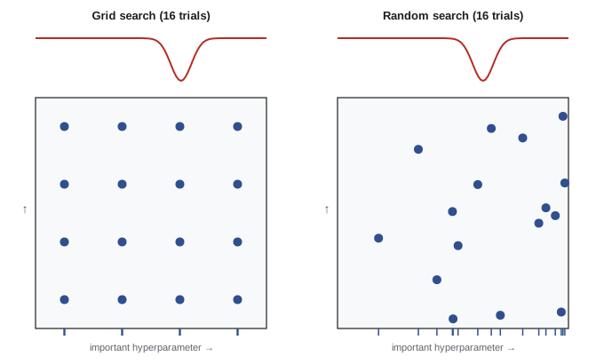
Grid search tries every combination of a few values per hyperparameter. It is simple, but its cost grows exponentially with the number of hyperparameters, and when only one of them matters, most trials repeat the same few values of it. Random search samples each hyperparameter independently from its range. With the same budget, it tries as many distinct values of each hyperparameter as there are trials, which is why it is usually better when the effective dimension is low.

import numpy as np

# Validation error depends strongly on log learning rate and weakly on log weight decay
def val_error(log_lr, log_wd):
    return 0.10 + 0.08 * (log_lr + 3.1) ** 2 + 0.002 * (log_wd + 4) ** 2

rng = np.random.default_rng(0)
budget = 16
lo_lr, hi_lr, lo_wd, hi_wd = -5.0, -1.0, -6.0, -2.0

# Grid: 4 x 4, so only 4 distinct learning rates are ever tried
g = np.linspace(0, 1, 4)
grid = [(lo_lr + a * (hi_lr - lo_lr), lo_wd + b * (hi_wd - lo_wd)) for a in g for b in g]
# Random: 16 distinct learning rates
rand = [(rng.uniform(lo_lr, hi_lr), rng.uniform(lo_wd, hi_wd)) for _ in range(budget)]

for name, pts in (("grid", grid), ("random", rand)):
    errs = [val_error(*p) for p in pts]
    i = int(np.argmin(errs))
    distinct = len({round(p[0], 6) for p in pts})
    print(f"{name:6s}: best error {errs[i]:.4f} at lr = 10^{pts[i][0]:.2f}, distinct learning rates tried {distinct}")

# Repeat random search many times to see the typical outcome
best = [min(val_error(rng.uniform(lo_lr, hi_lr), rng.uniform(lo_wd, hi_wd)) for _ in range(budget)) for _ in range(2000)]
print(f"random search, median best over 2000 repeats: {np.median(best):.4f}; optimum 0.1000")

grid  : best error 0.1266 at lr = 10^-3.67, distinct learning rates tried 4
random: best error 0.1121 at lr = 10^-2.83, distinct learning rates tried 16
random search, median best over 2000 repeats: 0.1026; optimum 0.1000

Quasi-random sequences (Sobol, Halton) spread points more evenly than independent random draws and can do slightly better still.

Bayesian optimization

Bayesian optimization builds a statistical model (a surrogate) of the objective from the trials so far and uses it to choose the next trial, balancing exploration (trying where uncertainty is high) and exploitation (trying where the predicted value is good). The classic surrogate is a Gaussian process (GP), which gives at each candidate point a predicted mean \(\mu(x)\) and standard deviation \(\sigma(x)\). An acquisition function turns these into a score; the most common is expected improvement over the best value so far, \(f^+\):

where \(\Phi\) and \(\phi\) are the standard normal distribution and density. EI is large where the mean is low (exploitation) or the uncertainty is high (exploration).

import numpy as np
from scipy.stats import norm

# Bayesian optimization of an expensive 1-D objective (validation loss against log learning rate)
def objective(x):
    return 0.3 + 0.1 * np.sin(3 * x) + 0.05 * (x + 3) ** 2

def kernel(a, b, ls=0.6, var=0.05):
    return var * np.exp(-0.5 * (a[:, None] - b[None, :]) ** 2 / ls ** 2)

def gp_posterior(xs, ys, xq, noise=1e-6):
    K = kernel(xs, xs) + noise * np.eye(len(xs))
    Ks = kernel(xs, xq)
    alpha = np.linalg.solve(K, ys - ys.mean())
    mu = ys.mean() + Ks.T @ alpha
    v = np.linalg.solve(K, Ks)
    var = np.clip(np.diag(kernel(xq, xq)) - np.sum(Ks * v, axis=0), 1e-12, None)
    return mu, np.sqrt(var)

grid = np.linspace(-5, -1, 801)
xs = np.array([-4.5, -1.5])
ys = objective(xs)
for it in range(8):
    mu, sd = gp_posterior(xs, ys, grid)
    best = ys.min()
    z = (best - mu) / sd
    ei = (best - mu) * norm.cdf(z) + sd * norm.pdf(z)       # expected improvement
    x_next = grid[np.argmax(ei)]
    xs, ys = np.append(xs, x_next), np.append(ys, objective(x_next))
    print(f"evaluation {it + 3}: try x = {x_next:6.3f}, loss {ys[-1]:.4f}, best so far {ys.min():.4f}")
print(f"true minimum on the grid: {objective(grid).min():.4f} at x = {grid[np.argmin(objective(grid))]:.3f}")

evaluation 3: try x = -3.665, loss 0.4221, best so far 0.3321
evaluation 4: try x = -5.000, loss 0.4350, best so far 0.3321
evaluation 5: try x = -2.595, loss 0.2084, best so far 0.2084
evaluation 6: try x = -2.325, loss 0.2590, best so far 0.2084
evaluation 7: try x = -2.830, loss 0.2210, best so far 0.2084
evaluation 8: try x = -2.660, loss 0.2066, best so far 0.2066
evaluation 9: try x = -1.000, loss 0.4859, best so far 0.2066
evaluation 10: try x = -2.660, loss 0.2066, best so far 0.2066
true minimum on the grid: 0.2066 at x = -2.655

Bayesian optimization is most valuable when each trial is very expensive and the number of hyperparameters is modest (up to roughly 10 to 20). For higher dimensions and mixed or conditional spaces, tree-based surrogates such as the tree-structured Parzen estimator (TPE, used in the Optuna and Hyperopt libraries) and random-forest surrogates (SMAC) are common. Batch versions propose several trials at once to use parallel workers.

Stopping bad trials early

Most of the cost of hyperparameter search is spent training configurations that turn out to be poor. Since a poor configuration is often recognizably poor early in training, multi-fidelity methods evaluate many configurations cheaply and give more resources only to promising ones.

• Successive halving: train \(n\) configurations for a small budget, keep the best fraction \(1/\eta\) (for example a third), multiply their budget by \(\eta\), and repeat until one remains.
• Hyperband runs several successive-halving brackets with different trade-offs between the number of configurations and the starting budget, hedging against the risk that early performance is misleading.
• ASHA (asynchronous successive halving) promotes configurations as soon as they qualify, keeping many parallel workers busy.
• BOHB and similar methods combine Bayesian proposals with Hyperband-style budgets.

import numpy as np

rng = np.random.default_rng(1)
# Each configuration has a final error and a learning curve that approaches it
n_configs = 81
final = 0.08 + 0.25 * rng.random(n_configs) ** 2
speed = rng.uniform(0.5, 2.0, n_configs)

def error_after(i, epochs):
    return final[i] + (0.9 - final[i]) * np.exp(-speed[i] * epochs / 10) + rng.normal(0, 0.005)

# Successive halving: start all configs with 1 epoch, keep the best third, triple their budget
alive, epochs, cost = list(range(n_configs)), 1, 0
while len(alive) > 1:
    scores = [(error_after(i, epochs), i) for i in alive]
    cost += epochs * len(alive)
    scores.sort()
    print(f"budget {epochs:3d} epochs: {len(alive):2d} configs, best so far {scores[0][0]:.3f}")
    alive = [i for _, i in scores[: max(1, len(alive) // 3)]]
    epochs *= 3
chosen = alive[0]
print(f"chosen config final error {final[chosen]:.3f}; true best {final.min():.3f}; rank {int(np.sum(final < final[chosen])) + 1} of {n_configs}")
print(f"epochs used {cost}, versus {n_configs * 81} to train every config for 81 epochs")

budget   1 epochs: 81 configs, best so far 0.751
budget   3 epochs: 27 configs, best so far 0.540
budget   9 epochs:  9 configs, best so far 0.232
budget  27 epochs:  3 configs, best so far 0.089
chosen config final error 0.089; true best 0.080; rank 14 of 81
epochs used 324, versus 6561 to train every config for 81 epochs

The output shows both the power and the weakness of early stopping. It used 324 epochs instead of 6,561, but the chosen configuration ranked 14th of 81: configurations that learn slowly but finish well were discarded after one epoch. Hyperband's multiple brackets, and starting budgets large enough to separate configurations, reduce this risk.

The learning rate deserves special care

The learning rate is usually the most important hyperparameter, and some practical tools help find it quickly:

• Learning-rate range test: train briefly while increasing the learning rate exponentially from very small to very large, and plot loss against learning rate. Loss falls, flattens, then diverges; a good maximum learning rate is somewhat below the point of divergence, often by a factor of three to ten.
• Schedules matter as much as values: warm-up for a few hundred to a few thousand steps, then cosine or linear decay, or a constant rate followed by a short cooldown (Lesson 3).
• Batch size and learning rate interact: with SGD, scaling the learning rate with batch size works up to a critical batch size (Lesson 3); with Adam, a square-root rule is a common starting point.
• Divergence early in training (loss spikes or NaNs) usually means the learning rate is too high or warm-up too short; slow, steady improvement may mean it is too low.

Transferring hyperparameters across scale

Tuning a large model directly is prohibitively expensive. A practical approach is to tune a small proxy model and transfer the settings. Standard parameterizations make this unreliable, because the best learning rate shifts as width grows. The maximal update parameterization (μP) rescales initializations, learning rates and output multipliers per layer so that, as width increases, each layer's updates stay the same size; then optimal hyperparameters found on a narrow model remain near-optimal for much wider ones ("μTransfer"). Combined with scaling laws (Lesson 9), which predict loss as a function of model size and data, this lets teams plan large training runs from small experiments.

Good practice

• Fix a budget and a protocol in advance; record every trial with its full configuration, code version, data version and random seed.
• Start broad and coarse, then narrow around good regions.
• Repeat the best few configurations with different seeds before declaring a winner; differences smaller than run-to-run variation are not real.
• Keep a held-out test set untouched by the search, and report results on it once.
• Prefer robust settings, those whose performance changes little nearby, over a sharp optimum.