Momentum, Adam and adaptive methods

Plain gradient descent has two weaknesses that Lesson 1 exposed. In ill-conditioned problems it zigzags across narrow valleys while crawling along them, needing a number of steps proportional to the condition number. And one learning rate must serve every parameter, even when different parameters see gradients that differ by orders of magnitude, as they do across the layers of a deep network. Momentum addresses the first problem by accumulating velocity along consistent directions; adaptive methods address the second by giving each parameter its own effective step size. Adam combines both, and with its weight-decay variant AdamW it is the default optimizer for transformers and most of modern deep learning.

Momentum

The heavy-ball method, due to Boris Polyak (1964), adds a fraction of the previous step to the current one:

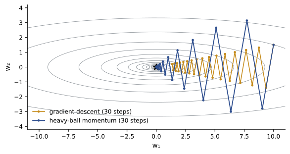
with momentum coefficient \(\beta\) typically 0.9. The velocity \(\mathbf{v}\) is an exponentially weighted sum of past gradients. Along a direction where the gradient keeps the same sign, such as the long axis of a valley, contributions accumulate, and the effective step approaches \(\eta/(1 - \beta)\), ten times \(\eta\) for \(\beta = 0.9\). Across the valley, where the gradient alternates in sign, contributions cancel and the zigzag is damped. Deep learning frameworks usually implement SGD with momentum in the equivalent form \(\mathbf{v} \leftarrow \beta\mathbf{v} + \mathbf{g}\), \(\mathbf{w} \leftarrow \mathbf{w} - \eta\mathbf{v}\).

On a strongly convex quadratic, heavy ball with optimal parameters, \(\eta = 4/(\sqrt{L} + \sqrt{\mu})^2\) and \(\beta = \big((\sqrt\kappa - 1)/(\sqrt\kappa + 1)\big)^2\), contracts the error by a factor of about \((\sqrt\kappa - 1)/(\sqrt\kappa + 1)\) per step, so the number of iterations scales with \(\sqrt\kappa\) instead of \(\kappa\). For \(\kappa = 10{,}000\) that is the difference between about 100 and 10,000 times \(\ln(1/\varepsilon)\).

Nesterov acceleration

Yurii Nesterov's accelerated gradient method (1983) evaluates the gradient at a look-ahead point:

The gradient at the point momentum is about to carry the iterate to acts as a correction before overshooting. Nesterov's method provably achieves the \(\sqrt\kappa\) dependence for all smooth strongly convex functions, and for smooth convex functions improves gradient descent's \(O(1/k)\) rate to \(O(1/k^2)\), which is optimal among first-order methods. In deep learning, the practical difference between heavy ball and Nesterov momentum is usually small.

import numpy as np

rng = np.random.default_rng(0)
Q, _ = np.linalg.qr(rng.normal(size=(50, 50)))
eigs = np.logspace(0, 2, 50)                       # curvatures 1 to 100, kappa = 100
A = Q @ np.diag(eigs) @ Q.T
w0 = rng.normal(size=50)
L, mu = eigs.max(), eigs.min()

def run(method, tol=1e-6, max_iter=5000):
    w, v = w0.copy(), np.zeros(50)
    e0 = np.linalg.norm(w0)
    for k in range(1, max_iter + 1):
        if method == "gd":
            w = w - 2 / (L + mu) * (A @ w)
        else:
            sk = np.sqrt(L / mu)
            if method == "heavy ball":                # optimal heavy-ball parameters for a quadratic
                eta, beta = 4 / (np.sqrt(L) + np.sqrt(mu)) ** 2, ((sk - 1) / (sk + 1)) ** 2
            else:                                     # standard Nesterov parameters
                eta, beta = 1 / L, (sk - 1) / (sk + 1)
            point = w + beta * v if method == "nesterov" else w
            v = beta * v - eta * (A @ point)
            w = w + v
        if np.linalg.norm(w) < tol * e0:
            return k
    return max_iter

for m in ["gd", "heavy ball", "nesterov"]:
    print(f"{m:11s} iterations to reduce error by 1e6: {run(m)}")

gd          iterations to reduce error by 1e6: 604
heavy ball  iterations to reduce error by 1e6: 86
nesterov    iterations to reduce error by 1e6: 125

Adaptive learning rates

Adaptive methods scale each coordinate's step by the inverse of a running estimate of that coordinate's gradient magnitude, a form of diagonal preconditioning learned from the gradients:

• AdaGrad (Duchi, Hazan and Singer, 2011) divides by the square root of the sum of all past squared gradients, so coordinates with large or frequent gradients get small steps and rare features get large ones. It works well for sparse problems, but its effective step only shrinks, which can stall long training runs.
• RMSProp (Hinton, 2012) replaces the sum with an exponential moving average, \(\mathbf{s} \leftarrow \rho\mathbf{s} + (1 - \rho)\mathbf{g}^2\) (elementwise), and steps by \(\eta\,\mathbf{g}/(\sqrt{\mathbf{s}} + \epsilon)\), so the step adapts to recent gradient magnitudes without decaying forever.

Adam

Adam (Kingma and Ba, 2015) combines momentum with RMSProp-style scaling. With gradient \(\mathbf{g}_t\) at step \(t\), it maintains moving averages of the gradient and its elementwise square, corrects them for their initialization at zero, and steps:

Default hyperparameters are \(\beta_1 = 0.9\), \(\beta_2 = 0.999\) and \(\epsilon = 10^{-8}\); large language model training often uses \(\beta_2 = 0.95\) for faster adaptation. Because the step for each coordinate is the ratio of a mean to a root-mean-square, its magnitude is roughly \(\eta\) regardless of the gradient's scale: Adam is approximately invariant to rescaling the gradient of each parameter. That robustness to scale, across layers and parameter types, is the main reason it trains transformers far more reliably than plain SGD.

The bias correction matters early in training. Since \(\mathbf{m}_0 = \mathbf{0}\), after one step \(\mathbf{m}_1 = 0.1\,\mathbf{g}_1\), a tenth of the gradient; dividing by \(1 - 0.9^1 = 0.1\) restores it. For \(\mathbf{v}\), with \(\beta_2 = 0.999\), the uncorrected average would be a thousandth of the true value at first, making early steps much too large; correction prevents that.

import numpy as np

def rosenbrock(w):
    x, y = w
    f = (1 - x) ** 2 + 100 * (y - x * x) ** 2
    g = np.array([-2 * (1 - x) - 400 * x * (y - x * x), 200 * (y - x * x)])
    return f, g

def optimize(method, lr, steps=5000):
    w = np.array([-1.5, 2.0])
    m = np.zeros(2); v = np.zeros(2)
    for t in range(1, steps + 1):
        f, g = rosenbrock(w)
        if not np.isfinite(f) or f > 1e12:
            return float("inf")
        if method == "sgd":
            w = w - lr * g
        elif method == "momentum":
            m = 0.9 * m + g
            w = w - lr * m
        else:                                   # adam
            m = 0.9 * m + 0.1 * g
            v = 0.999 * v + 0.001 * g * g
            m_hat = m / (1 - 0.9 ** t); v_hat = v / (1 - 0.999 ** t)
            w = w - lr * m_hat / (np.sqrt(v_hat) + 1e-8)
    return rosenbrock(w)[0]

for method, lrs in [("sgd", [1e-4, 1e-3, 1e-2]), ("momentum", [1e-5, 1e-4, 1e-3]), ("adam", [1e-3, 1e-2, 1e-1])]:
    res = "  ".join(f"lr={lr:g}: {optimize(method, lr):.2e}" for lr in lrs)
    print(f"{method:9s} {res}")

sgd       lr=0.0001: 4.48e+00  lr=0.001: 6.51e-03  lr=0.01: inf
momentum  lr=1e-05: 4.49e+00  lr=0.0001: 6.38e-03  lr=0.001: 1.99e-19
adam      lr=0.001: 1.12e+00  lr=0.01: 1.68e-17  lr=0.1: 1.09e-08

The Rosenbrock function has a long, curved, narrow valley, a classic test of optimizers. Plain gradient descent diverges at a learning rate of 0.01 and is still far from the minimum at 10⁻⁴. Momentum, well tuned, does extremely well here, but its useful range is shifted about tenfold lower than plain gradient descent's, because momentum multiplies the effective step. Adam reaches very low loss at two of the three rates and is still descending at the third. Every method has a window of workable learning rates; the practical advantage of Adam is that its window depends far less on the scale of each parameter's gradient, which in a deep network varies by orders of magnitude between layers.

Weight decay and AdamW

Weight decay shrinks parameters toward zero at each step, \(\mathbf{w} \leftarrow \mathbf{w} - \eta\lambda\mathbf{w}\), as a regularizer. For plain SGD, this is identical to adding an L2 penalty \(\tfrac{\lambda}{2}\|\mathbf{w}\|^2\) to the loss. For Adam it is not: an L2 penalty adds \(\lambda\mathbf{w}\) to the gradient, which then gets divided by \(\sqrt{\hat{\mathbf{v}}}\), so parameters with large gradient variance are barely regularized while those with small gradients are regularized heavily. Loshchilov and Hutter (2019) showed that decoupling the decay from the adaptive scaling, AdamW, regularizes better:

AdamW with weight decay of about 0.01 to 0.1, warmup and cosine or linear decay is the standard recipe for transformers. Biases and normalization parameters are usually excluded from weight decay.

Practical matters

Gradient clipping

Occasional very large gradients, from a bad batch, a numerical spike or a sharp region of the loss surface, can throw a model far off course in one step. Gradient clipping rescales the whole gradient when its norm exceeds a threshold \(c\): \(\mathbf{g} \leftarrow \mathbf{g}\cdot\min(1, c/\|\mathbf{g}\|)\). A threshold of 1.0 is common in transformer training. Clipping by global norm preserves the gradient's direction, unlike clipping each coordinate.

Memory

Adam stores two extra values per parameter, \(\mathbf{m}\) and \(\mathbf{v}\), in addition to the parameters and gradients. For large models, optimizer state is a major part of memory.

Choosing an optimizer

For transformers and most new architectures, AdamW with warmup and decay is the reliable default. For convolutional networks on image classification, SGD with momentum (0.9), weight decay and a step or cosine schedule remains competitive and sometimes generalizes slightly better. Research continues: newer optimizers such as Lion (which uses only the sign of a momentum term), Shampoo (which uses larger, non-diagonal preconditioners per layer) and Muon (which orthogonalizes the updates of matrix-shaped parameters) have shown gains in some large-scale settings, but none has yet displaced AdamW as the general default. Whatever the optimizer, the learning rate and its schedule matter more than the choice between well-tuned alternatives.

Lesson 6 shows how the gradients these optimizers consume are computed, and Lesson 8 how the choice of optimizer affects which solution is found and how well it generalizes.