Stochastic gradient methods

The loss functions of machine learning are averages over training examples. Computing the exact gradient of such an average means passing over the entire data set, which for millions of images or trillions of text tokens is far too expensive to do at every step. Stochastic gradient descent (SGD) instead estimates the gradient from a small random sample, a minibatch, and takes a step based on that noisy estimate. Each step is cheap and imprecise, but with the right step sizes the noise averages out. SGD and its variants are how essentially every neural network is trained.

This lesson defines the stochastic gradient and its variance, explains how batch size and learning rate interact, covers learning rate schedules and the conditions for convergence, and describes practical matters such as epochs, shuffling, gradient accumulation and variance reduction.

Empirical risk and the stochastic gradient

With training examples \((\mathbf{x}_i, y_i)\), \(i = 1, \ldots, n\), and a per-example loss \(\ell_i(\mathbf{w}) = \ell(\mathbf{w}; \mathbf{x}_i, y_i)\), training minimizes the empirical risk

A minibatch \(B\) of \(b\) examples drawn uniformly at random gives the stochastic gradient

It is an unbiased estimate of the full gradient: right on average, wrong in any single draw. If the per-example gradients have covariance with total variance \(\sigma^2\) (the trace of the covariance), the minibatch gradient's variance is \(\sigma^2/b\) when sampling with replacement, so its typical error falls as \(1/\sqrt{b}\). SGD then iterates \(\mathbf{w}_{k+1} = \mathbf{w}_k - \eta_k\,\mathbf{g}(\mathbf{w}_k)\).

import numpy as np

rng = np.random.default_rng(0)
n, d = 20000, 10
X = rng.normal(size=(n, d))
y = X @ rng.normal(size=d) + rng.normal(scale=2.0, size=n)
w = np.zeros(d)                                   # evaluate gradients at w = 0
full = X.T @ (X @ w - y) / n

for b in [1, 8, 64, 512]:
    errs = []
    for _ in range(2000):
        idx = rng.integers(0, n, size=b)
        g = X[idx].T @ (X[idx] @ w - y[idx]) / b
        errs.append(np.sum((g - full) ** 2))
    print(f"batch {b:4d}: mean squared error of gradient = {np.mean(errs):8.3f}")

batch    1: mean squared error of gradient =  207.754
batch    8: mean squared error of gradient =   27.707
batch   64: mean squared error of gradient =    3.420
batch  512: mean squared error of gradient =    0.433

Each eightfold increase in batch size cuts the gradient's mean squared error about eightfold. But the cost per step also rises eightfold, so whether a larger batch is worthwhile depends on whether the noise or the curvature is limiting progress, a question taken up below.

Why noise helps and hurts

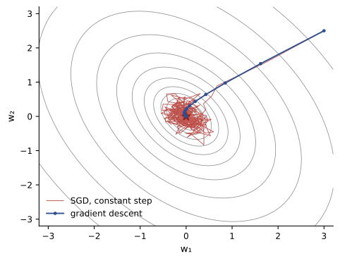
Gradient noise has three effects. First, it makes each step cheap, so SGD makes progress long before a full-batch method has finished computing one gradient; on redundant data sets, a minibatch gradient is nearly as informative as the full one. Second, it prevents exact convergence with a constant step size: near the minimum the true gradient is small but the noise is not, so the iterates bounce around the minimum in a region whose size is proportional to \(\eta\sigma^2\), the noise floor. Third, in non-convex problems, noise can help the iterates escape saddle points and sharp minima (Lesson 9).

For a \(\mu\)-strongly convex, \(L\)-smooth objective with gradient noise variance \(\sigma^2\), SGD with a constant step \(\eta \le 1/L\) satisfies roughly

The first term decays linearly, as in gradient descent; the second is the noise floor, which does not decay. Halving the step size halves the floor but slows the linear phase. This trade-off is why learning rates are decreased during training.

Step-size conditions and rates

To converge exactly, the step sizes must shrink, but not too fast. The classical Robbins-Monro conditions are

The first ensures the iterates can travel any distance; the second ensures the accumulated noise is finite. Steps \(\eta_k = c/(k + k_0)\) satisfy both. With such schedules, SGD reaches expected error \(O(1/k)\) for strongly convex problems and \(O(1/\sqrt{k})\) for general convex ones (with suitable averaging of the iterates). These rates are slower than gradient descent per iteration, but each iteration costs \(b\) gradient evaluations instead of \(n\), and the rates do not depend on \(n\) at all, which is decisive for large data sets.

import numpy as np

rng = np.random.default_rng(1)
n, d = 5000, 5
X = rng.normal(size=(n, d))
w_star = rng.normal(size=d)
y = X @ w_star + rng.normal(scale=1.0, size=n)
w_opt = np.linalg.lstsq(X, y, rcond=None)[0]

def sgd(schedule, steps=20000, b=4, seed=2):
    r = np.random.default_rng(seed)
    w = np.zeros(d)
    out = {}
    for k in range(1, steps + 1):
        idx = r.integers(0, n, size=b)
        g = X[idx].T @ (X[idx] @ w - y[idx]) / b
        w -= schedule(k) * g
        if k in (100, 1000, 5000, 20000):
            out[k] = np.sum((w - w_opt) ** 2)
    return out

runs = {
    "constant 0.05": lambda k: 0.05,
    "constant 0.005": lambda k: 0.005,
    "decay 0.05*100/(k+100)": lambda k: 0.05 * 100 / (k + 100),
}
print("steps:                       100      1000      5000     20000")
for name, s in runs.items():
    r = sgd(s)
    print(f"{name:24s}" + "".join(f"{r[k]:10.2e}" for k in (100, 1000, 5000, 20000)))

steps:                       100      1000      5000     20000
constant 0.05             2.14e-02  9.53e-02  2.55e-02  1.79e-02
constant 0.005            1.38e+00  1.14e-02  1.85e-03  3.11e-03
decay 0.05*100/(k+100)    2.60e-02  1.27e-02  7.52e-04  2.18e-04

The large constant step makes fast early progress, then stalls at its noise floor. The small constant step has a lower floor but is slow at first. The decaying schedule starts fast and keeps improving, combining the advantages of both.

Learning rate schedules in practice

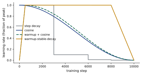
Deep learning practice uses a few standard schedules, usually expressed per optimizer step:

• Step decay: multiply the learning rate by a factor (often 0.1) at fixed points, for example after 30, 60 and 80 of 90 epochs, the classic schedule for training ResNets on ImageNet.
• Cosine decay: \(\eta_k = \eta_{\min} + \tfrac12(\eta_{\max} - \eta_{\min})(1 + \cos(\pi k/K))\) over \(K\) steps, a smooth decrease from the peak to a small final value. It is the default for many vision and language models.
• Linear warmup: start from a small value and increase linearly to the peak over the first few hundred or thousand steps. Warmup prevents instability at the start of training, when the parameters are far from any good region, gradients can be large, and adaptive optimizers (Lesson 5) have poor estimates of gradient statistics. Almost all transformer training uses warmup followed by cosine or linear decay.
• Warmup-stable-decay: warm up, hold a constant rate for most of training, then decay rapidly at the end. It allows training to be extended or checkpoints reused, and has become common for large language models.

Batch size and learning rate

A larger batch gives a less noisy gradient, so it can tolerate a larger step. For moderate batch sizes, the linear scaling rule works well empirically: when the batch size is multiplied by \(k\), multiply the learning rate by \(k\), keeping the number of epochs (passes over the data) fixed. Each step then makes roughly \(k\) times the progress of a small-batch step, so the total number of examples processed, and the result, stay about the same while the number of steps falls by \(k\), which is what allows training to be spread across many accelerators.

The rule breaks down above a problem-dependent critical batch size. Beyond it, the gradient is already accurate enough that curvature, not noise, limits the step size (the step cannot exceed about \(2/L\) however clean the gradient), so larger batches give diminishing returns: more computation for little reduction in steps. The critical batch size grows as training progresses and the loss falls, and is larger for harder tasks; it is one reason large language models use batches of millions of tokens.

import numpy as np

rng = np.random.default_rng(3)
n, d = 50000, 20
scales = np.linspace(0.3, 3.0, d)                 # curvatures from 0.09 to 9
X = rng.normal(size=(n, d)) * scales
y = X @ rng.normal(size=d) + rng.normal(scale=3.0, size=n)
w_opt = np.linalg.lstsq(X, y, rcond=None)[0]
L = np.max(scales ** 2)

def steps_to_target(b, eta, target=0.05, max_steps=200000):
    w = np.zeros(d)
    for k in range(1, max_steps + 1):
        idx = rng.integers(0, n, size=b)
        w -= eta * X[idx].T @ (X[idx] @ w - y[idx]) / b
        if k % 10 == 0 and np.sum((w - w_opt) ** 2) < target:
            return k
    return None

base_b, base_eta = 8, 0.002
for b in [8, 32, 128, 512, 2048]:
    eta = min(base_eta * b / base_b, 1.0 / L)       # linear scaling, capped by curvature
    k = steps_to_target(b, eta)
    print(f"batch {b:5d}  lr {eta:.4f}  steps {k:6d}  examples {k * b:8d}")

batch     8  lr 0.0020  steps   3900  examples    31200
batch    32  lr 0.0080  steps    900  examples    28800
batch   128  lr 0.0320  steps    210  examples    26880
batch   512  lr 0.1111  steps     90  examples    46080
batch  2048  lr 0.1111  steps     70  examples   143360

Up to a batch of about 128, multiplying the batch by four cuts the steps by about four, with roughly constant total examples. Beyond that, the learning rate hits the curvature limit \(1/L\), the number of steps stops falling much, and the total computation grows: the batch has passed its critical size.

Epochs, shuffling and accumulation

In practice minibatches are drawn without replacement: the data set is shuffled and divided into consecutive batches, and one pass over all of it is an epoch. Shuffling again each epoch (random reshuffling) usually converges somewhat faster than sampling with replacement, and avoids the systematic bias of a fixed order, such as all examples of one class arriving together.

When the desired batch does not fit in accelerator memory, gradient accumulation computes gradients for several smaller micro-batches, adds them, and takes one optimizer step. Accumulating 8 micro-batches of 32 is mathematically equivalent to one batch of 256 (apart from layers, such as batch normalization, whose statistics depend on the micro-batch), at the cost of more time per step. Data parallelism across devices achieves the same effect by averaging gradients computed on different devices.

Variance reduction

For finite sums, a family of methods removes the noise floor without shrinking the step. SVRG (stochastic variance reduced gradient) periodically computes a full gradient \(\nabla F(\tilde{\mathbf{w}})\) at a snapshot point and then uses

which is still unbiased but whose variance shrinks to zero as both \(\mathbf{w}\) and \(\tilde{\mathbf{w}}\) approach the optimum. SVRG, SAGA and related methods achieve linear convergence on strongly convex finite sums with constant steps. They are powerful for convex problems such as large-scale logistic regression, but have had little success in deep learning, where the snapshot gradient quickly becomes stale and the cost of full passes is high.

Lesson 4 adds curvature with Newton and quasi-Newton methods, and Lesson 12 returns to batch size when training is spread across many devices.