
AI-310 · Lesson 7 of 12 · 31 min
Constrained and convex optimization
Many problems in machine learning come with constraints or non-smooth terms: weights that must be non-negative, probabilities that must sum to one, a margin that must be met, a fairness criterion that must hold, or an L1 penalty whose kink at zero is what makes solutions sparse. And many important problems are convex, which means they can be solved to global optimality, reliably and with certificates of how close a solution is to the best possible. This lesson develops the tools for these problems: convex problem structure, Lagrangian duality and the KKT conditions, projected and proximal gradient methods, and the role of general-purpose convex solvers.
Convex optimization problems
A convex optimization problem has the form
where the objective \(f_0\) and inequality constraint functions \(f_i\) are convex and the equality constraints are affine. The feasible set is then convex, and the fundamental property follows: every local minimum is a global minimum. There is no risk of being trapped in a poor solution, and an algorithm's progress can be measured against the true optimum.
Recognizing convexity is a skill. Useful building blocks are affine functions, norms, \(e^x\), \(-\log x\), \(x^2\) and other powers \(|x|^p\) with \(p \ge 1\), the log-sum-exp function \(\log\sum e^{x_i}\), and quadratic forms \(\mathbf{x}^\top Q\mathbf{x}\) with \(Q\) positive semidefinite. Convexity is preserved by non-negative weighted sums, composition with affine maps, and pointwise maxima. So the logistic regression loss (a sum of log-sum-exp terms of affine functions), the hinge loss of support vector machines (a maximum of affine functions), least squares, and their sums with norm penalties are all convex.
| Problem | Objective | Constraints | Class |
|---|---|---|---|
| Least squares | ‖Xw − y‖² | none | Quadratic |
| Lasso | ‖Xw − y‖² + λ‖w‖₁ | none (non-smooth) | Convex, non-smooth |
| Non-negative least squares | ‖Xw − y‖² | w ≥ 0 | Quadratic program |
| Support vector machine | ½‖w‖² + C Σξᵢ | yᵢ(wᵀxᵢ + b) ≥ 1 − ξᵢ, ξ ≥ 0 | Quadratic program |
| Logistic regression | Σ log(1 + e^(−yᵢwᵀxᵢ)) | none | Smooth convex |
| Resource allocation | cᵀw | Aw ≤ b, w ≥ 0 | Linear program |
Lagrangian duality
Constraints are handled by introducing a Lagrange multiplier for each one. The Lagrangian is
and the dual function \(g(\boldsymbol\lambda, \boldsymbol\nu) = \min_{\mathbf{w}}\mathcal{L}\) gives a lower bound on the optimal value \(p^*\) for any \(\boldsymbol\lambda \ge 0\): for a feasible \(\mathbf{w}\), each \(\lambda_i f_i \le 0\) and the equality term vanishes, so \(\mathcal{L} \le f_0\). Maximizing that bound gives the dual problem, whose optimal value \(d^*\) satisfies weak duality, \(d^* \le p^*\). For convex problems satisfying a mild regularity condition, Slater's condition (there is a strictly feasible point), strong duality holds: \(d^* = p^*\).
Duality is practical, not only theoretical. The duality gap \(f_0(\mathbf{w}) - g(\boldsymbol\lambda, \boldsymbol\nu)\) between any feasible primal point and any dual point bounds how far the primal point is from optimal, giving a rigorous stopping criterion. The multipliers have meaning: \(\lambda_i^*\) is the rate at which the optimal value would improve if constraint \(i\) were relaxed, the shadow price of that constraint. And some problems are easier in their dual form: the dual of the support vector machine depends on the data only through inner products \(\mathbf{x}_i^\top\mathbf{x}_j\), which is what allows kernels.
The KKT conditions
For a convex problem with strong duality, a point \(\mathbf{w}^*\) is optimal, with multipliers \(\boldsymbol\lambda^*, \boldsymbol\nu^*\), exactly when the Karush-Kuhn-Tucker conditions hold:
- Stationarity: \(\nabla f_0(\mathbf{w}^*) + \sum_i\lambda_i^*\nabla f_i(\mathbf{w}^*) + A^\top\boldsymbol\nu^* = \mathbf{0}\).
- Primal feasibility: \(f_i(\mathbf{w}^*) \le 0\) and \(A\mathbf{w}^* = \mathbf{b}\).
- Dual feasibility: \(\boldsymbol\lambda^* \ge 0\).
- Complementary slackness: \(\lambda_i^* f_i(\mathbf{w}^*) = 0\) for every \(i\).
Complementary slackness says that each constraint is either active (holding with equality) or has a zero multiplier: a constraint that is not tight exerts no force. In the support vector machine, the training points with non-zero multipliers are exactly those on or inside the margin, the support vectors, which is why the solution depends only on them.
Worked problem
Solving a constrained problem with KKT
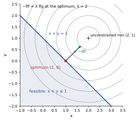
Minimize \((x - 2)^2 + (y - 1)^2\) subject to \(x + y \le 1\).
Show solution
- The unconstrained minimum (2, 1) violates \(x + y \le 1\), so the constraint is active: \(x + y = 1\), with \(\lambda > 0\).
- Stationarity: \(2(x - 2) + \lambda = 0\) and \(2(y - 1) + \lambda = 0\), so \(x - 2 = y - 1\), i.e. \(x = y + 1\).
- With \(x + y = 1\): \(y = 0\), \(x = 1\), and \(\lambda = -2(1 - 2) = 2 \ge 0\). All KKT conditions hold.
- Optimal value: \((1 - 2)^2 + (0 - 1)^2 = 2\).
Answer: The optimum is (1, 0) with value 2 and multiplier λ = 2: relaxing the constraint to \(x + y \le 1 + \delta\) would lower the optimal value by about \(2\delta\). Geometrically, (1, 0) is the projection of (2, 1) onto the half-plane.
import numpy as np
from scipy.optimize import minimize

f = lambda z: (z[0] - 2) ** 2 + (z[1] - 1) ** 2
grad = lambda z: np.array([2 * (z[0] - 2), 2 * (z[1] - 1)])
con = {"type": "ineq", "fun": lambda z: 1 - z[0] - z[1]}     # SciPy convention: fun(z) >= 0

res = minimize(f, x0=[0.0, 0.0], jac=grad, constraints=[con], method="SLSQP")
z = res.x
lam = -grad(z)[0]                                              # stationarity: grad f + lam * [1, 1] = 0
print(f"solution  x = {z[0]:.4f}, y = {z[1]:.4f}, f = {res.fun:.4f}")
print(f"multiplier from stationarity: lambda = {lam:.4f}")
print(f"constraint value x + y - 1 = {z.sum() - 1:.2e} (active)")

for delta in [0.1, 0.01]:
    con_d = {"type": "ineq", "fun": lambda z, d=delta: 1 + d - z[0] - z[1]}
    r = minimize(f, x0=[0.0, 0.0], jac=grad, constraints=[con_d], method="SLSQP")
print(f"relax by {delta}: optimum falls by {res.fun - r.fun:.4f} (lambda * delta = {lam * delta:.4f})")solution x = 1.0000, y = 0.0000, f = 2.0000 multiplier from stationarity: lambda = 2.0000 constraint value x + y - 1 = 7.11e-15 (active) relax by 0.1: optimum falls by 0.1950 (lambda * delta = 0.2000) relax by 0.01: optimum falls by 0.0199 (lambda * delta = 0.0200)
For small relaxations the decrease is close to \(\lambda\delta\); the small discrepancy is the second-order term, \(\delta^2/2\) here.
Linear programs and shadow prices
A linear program (LP) has a linear objective and linear constraints. LPs are solved routinely with millions of variables by the simplex method and interior-point methods, and their dual variables are the shadow prices of the constraints. Although less central to model training, LPs appear throughout operations research, in scheduling, capacity planning and transport, and as components of machine learning methods such as optimal transport.
from scipy.optimize import linprog

# Allocate GPU-hours (x1: training jobs, x2: inference jobs) to maximize value.
# value per unit: training 3, inference 2  ->  minimize the negative
c = [-3, -2]
A_ub = [[1, 1],        # total GPU-hours available: 100
        [2, 1],        # power budget units: 150
        [0, 1]]        # inference capped by demand: 80
b_ub = [100, 150, 80]
res = linprog(c, A_ub=A_ub, b_ub=b_ub, bounds=[(0, None), (0, None)], method="highs")
print(f"x1 = {res.x[0]:.1f}, x2 = {res.x[1]:.1f}, value = {-res.fun:.1f}")
print("shadow prices (value per extra unit of each resource):",
[round(float(-m), 3) for m in res.ineqlin.marginals])x1 = 50.0, x2 = 50.0, value = 250.0 shadow prices (value per extra unit of each resource): [1.0, 1.0, 0.0]
The solution uses all the GPU-hours and all the power budget, so both have positive shadow prices: one more GPU-hour would add 1 unit of value and one more unit of power 1 unit. The inference demand cap is not binding, so its shadow price is zero, an instance of complementary slackness.
Projected gradient descent
For a problem \(\min f(\mathbf{w})\) over a convex set \(C\), projected gradient descent takes a gradient step and then projects back onto the set:
It keeps the convergence rates of gradient descent, provided the projection is cheap. Many useful sets have simple projections:
- Box \(l \le w \le u\): clip each coordinate, \(\Pi(z)_i = \min(\max(z_i, l_i), u_i\)); for non-negativity, \(\max(z, 0)\).
- Euclidean ball \(\|\mathbf{w}\| \le r\): scale down if outside, \(\mathbf{z}\cdot\min(1, r/\|\mathbf{z}\|)\), the same operation as gradient clipping.
- Probability simplex \(\{\mathbf{w} \ge 0, \sum w_i = 1\}\): a sort-based algorithm finds a threshold \(\tau\) and sets \(w_i = \max(z_i - \tau, 0)\).
- Affine set \(\{A\mathbf{w} = \mathbf{b}\}\): \(\mathbf{z} - A^\top(AA^\top)^{-1}(A\mathbf{z} - \mathbf{b})\).
import numpy as np
from scipy.optimize import nnls

rng = np.random.default_rng(0)
X = rng.normal(size=(200, 6))
w_true = np.array([2.0, 0.0, 1.0, 0.0, 0.5, 0.0])
y = X @ w_true + 0.3 * rng.normal(size=200)

L = np.linalg.eigvalsh(X.T @ X).max()
w = np.zeros(6)
for k in range(2000):
    w = np.maximum(w - (1 / L) * X.T @ (X @ w - y), 0.0)        # gradient step, then project onto w >= 0

w_ref, _ = nnls(X, y)
w_ls = np.linalg.lstsq(X, y, rcond=None)[0]
print("projected GD:      ", np.round(w, 3))
print("scipy nnls:        ", np.round(w_ref, 3))
print("unconstrained LS: ", np.round(w_ls, 3))projected GD: [1.99 0.01 1.014 0.024 0.52 0. ] scipy nnls: [1.99 0.01 1.014 0.024 0.52 0. ] unconstrained LS: [ 1.995 0.013 1.02 0.023 0.521 -0.072]
Projected gradient descent matches the reference solver. Unconstrained least squares gives a small negative value (−0.072) for the last coefficient, whose true value is zero; the constraint holds it at exactly zero, the constrained optimum when the effects are known to be non-negative.
Proximal gradient methods and the lasso
Some objectives are a smooth part plus a non-smooth but simple part: \(F(\mathbf{w}) = f(\mathbf{w}) + h(\mathbf{w})\), such as a loss plus an L1 penalty. The gradient of \(h\) may not exist, but its proximal operator is easy:
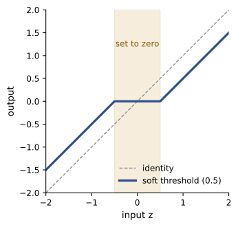
The proximal gradient method alternates a gradient step on \(f\) with a proximal step on \(h\): \(\mathbf{w}_{k+1} = \text{prox}_{\eta h}(\mathbf{w}_k - \eta\nabla f(\mathbf{w}_k))\). When \(h\) is the indicator of a convex set, the proximal operator is the projection, so projected gradient descent is a special case. For \(h(\mathbf{w}) = \lambda\|\mathbf{w}\|_1\), the proximal operator is soft thresholding, applied coordinate by coordinate:
Values within \(\eta\lambda\) of zero are set exactly to zero, and larger values are shrunk toward zero by \(\eta\lambda\). Applied to the lasso, \(\min \tfrac{1}{2n}\|X\mathbf{w} - \mathbf{y}\|^2 + \lambda\|\mathbf{w}\|_1\), this is ISTA (iterative shrinkage-thresholding algorithm), which converges at \(O(1/k)\). Its accelerated version FISTA, which adds Nesterov-style momentum, converges at \(O(1/k^2)\).
Worked problem
Soft thresholding
Apply soft thresholding with threshold \(\eta\lambda = 0.5\) to \(\mathbf{z} = (2.0, -0.3, 0.7, -1.4, 0.1)\).
Show solution
- 2.0 → 1.5; −0.3 → 0 (|−0.3| < 0.5); 0.7 → 0.2; −1.4 → −0.9; 0.1 → 0.
Answer: (1.5, 0, 0.2, −0.9, 0). Two of five coordinates become exactly zero, which is how the L1 penalty produces sparse models.
import numpy as np

rng = np.random.default_rng(1)
n, d = 80, 120                                    # more features than examples
Z = rng.normal(size=(n, d))
X = Z.copy()
for j in range(1, d):                             # adjacent features are correlated
    X[:, j] = 0.8 * X[:, j - 1] + 0.6 * Z[:, j]
w_true = np.zeros(d); w_true[[0, 25, 60, 100]] = [3.0, -2.0, 1.5, 1.0]
y = X @ w_true + 0.5 * rng.normal(size=n)
L = np.linalg.eigvalsh(X.T @ X / n).max()
soft = lambda z, t: np.sign(z) * np.maximum(np.abs(z) - t, 0.0)
obj = lambda w, lam: 0.5 / n * np.sum((X @ w - y) ** 2) + lam * np.abs(w).sum()

def ista(lam, iters, fast=False):
    w = np.zeros(d); z = w.copy(); t = 1.0
    for _ in range(iters):
        w_new = soft(z - (1 / L) * X.T @ (X @ z - y) / n, lam / L)
        if fast:
            t_new = (1 + np.sqrt(1 + 4 * t * t)) / 2
            z = w_new + (t - 1) / t_new * (w_new - w); t = t_new
        else:
            z = w_new
        w = w_new
    return w

for lam in [0.01, 0.1, 0.5]:
    w = ista(lam, 5000, fast=True)
    print(f"lambda {lam:4}: {np.sum(w != 0):2d} non-zero coefficients, largest: {np.round(np.sort(np.abs(w))[-4:][::-1], 2)}")

ref = obj(ista(0.1, 50000, fast=True), 0.1)
for iters in [10, 100, 1000]:
    gap_i = obj(ista(0.1, iters), 0.1) - ref
    gap_f = obj(ista(0.1, iters, fast=True), 0.1) - ref
print(f"{iters:4d} iterations: ISTA gap {gap_i:.2e} FISTA gap {gap_f:.2e}")lambda 0.01: 56 non-zero coefficients, largest: [2.91 1.94 1.46 0.9 ] lambda 0.1: 10 non-zero coefficients, largest: [2.88 1.9 1.44 0.89] lambda 0.5: 4 non-zero coefficients, largest: [2.64 1.46 1.03 0.65] 10 iterations: ISTA gap 1.15e+00 FISTA gap 7.15e-01 100 iterations: ISTA gap 8.16e-02 FISTA gap 3.11e-05 1000 iterations: ISTA gap 8.08e-12 FISTA gap 4.57e-14
At λ = 0.5 the lasso keeps exactly four coefficients, the four true features, shrunk somewhat toward zero; smaller λ keeps more. With correlated features and more features than examples, the problem is poorly conditioned: after 100 iterations FISTA is within 3 × 10⁻⁵ of the optimum while ISTA is still 0.08 away, the difference between O(1/k²) and O(1/k).
Solvers and modelling tools
For small and medium problems, general-purpose convex solvers based on interior-point methods find solutions to high accuracy in a few dozen iterations, each solving a linear system. Modelling libraries such as CVXPY let a problem be written almost as it appears on paper, check that it is convex by construction (disciplined convex programming), and pass it to a suitable solver. For very large problems, such as training on millions of examples, first-order methods like those in this lesson, often stochastic, are used instead, because each interior-point iteration becomes too expensive.
Convex optimization also appears inside non-convex deep learning: projections enforce constraints on parameters, proximal steps implement sparsity, and convex subproblems appear in methods such as constrained policy optimization in reinforcement learning (AI-330) and in certified robustness.
Lesson 11 extends constrained optimization to integer and combinatorial problems, where branch and bound builds on the linear programming relaxations of this lesson.
Common mistakes
MistakeAssuming a problem is convex because its objective is.
InsteadThe feasible set must also be convex: inequality functions convex, equalities affine.
MistakeApplying plain gradient descent to the L1 penalty.
InsteadIts subgradient oscillates and never yields exact zeros; use proximal gradient (soft thresholding).
MistakeIgnoring the sign of inequality multipliers.
InsteadMultipliers of ≤ constraints must be non-negative; a negative value signals an error or an inactive constraint.
MistakeStopping a convex solver on a fixed iteration count only.
InsteadUse the duality gap, which certifies how far the solution is from optimal.
MistakeMixing up solver sign conventions.
InsteadCheck whether a library expects g(x) ≤ 0 or g(x) ≥ 0, and minimization or maximization.
Summary and key terms
- Convex problems: convex objective, convex inequality constraints, affine equalities; every local minimum is global.
- Convexity is preserved by non-negative sums, affine composition and pointwise maxima; least squares, logistic, hinge and lasso objectives are convex.
- The Lagrangian and dual function give lower bounds (weak duality); Slater's condition gives strong duality.
- Duality gaps certify optimality; multipliers are shadow prices.
- KKT conditions: stationarity, primal and dual feasibility, complementary slackness.
- Projected gradient descent handles simple convex sets (boxes, balls, simplices, affine sets).
- Proximal gradient handles smooth + simple non-smooth objectives; soft thresholding gives the lasso (ISTA O(1/k), FISTA O(1/k²)).
- Interior-point solvers and modelling tools suit small and medium problems; first-order methods scale to large data.
- Convex optimization problem
- Minimizing a convex function over a convex set defined by convex inequalities and affine equalities.
- Lagrangian
- The objective plus multiplier-weighted constraint functions.
- Dual function
- The minimum of the Lagrangian over the primal variables, a lower bound on the optimum.
- Weak duality
- The dual optimum is never larger than the primal optimum.
- Strong duality
- The dual and primal optima are equal.
- Slater's condition
- Existence of a strictly feasible point, which guarantees strong duality for convex problems.
- Duality gap
- The difference between a primal objective value and a dual value.
- KKT conditions
- Necessary and (for convex problems) sufficient optimality conditions with multipliers.
- Complementary slackness
- Each constraint is active or has a zero multiplier.
- Shadow price
- The rate of improvement in the optimal value per unit relaxation of a constraint.
- Projection
- The closest point in a set to a given point.
- Proximal operator
- The minimizer of a function plus a quadratic distance penalty.
- Soft thresholding
- The proximal operator of the L1 norm: shrink toward zero, setting small values to zero.
- ISTA and FISTA
- Proximal gradient methods for L1-penalized problems, unaccelerated and accelerated.
Practice problems
Work each problem on paper first, then reveal the answer to check.
Is f(w) = max(0, 1 − w) + w² convex? Why?
Show answer
Yes: the hinge is a maximum of affine functions (convex), w² is convex, and sums of convex functions are convex.
Minimize x² + y² subject to x + y = 2 using a multiplier.
Show answer
Stationarity 2x + ν = 0, 2y + ν = 0 gives x = y = 1, ν = −2; optimal value 2.
Minimize (x − 3)² subject to x ≤ 1. What is the multiplier?
Show answer
Active: x = 1; stationarity 2(1 − 3) + λ = 0 gives λ = 4.
For the previous problem, by how much does the optimum change if the constraint becomes x ≤ 1.1?
Show answer
About λδ = 0.4 lower (exactly 4 − 3.61 = 0.39).
Project z = (3, −1, 0.5) onto the box [0, 1]³.
Show answer
(1, 0, 0.5).
Project z = (3, 4) onto the ball of radius 1.
Show answer
‖z‖ = 5; (0.6, 0.8).
Soft-threshold (0.8, −2.5, 0.2) with threshold 1.
Show answer
(0, −1.5, 0).
A constraint has multiplier zero at the optimum. What does complementary slackness imply?
Show answer
Either the constraint is inactive (slack), or it is active but not exerting force; relaxing it slightly does not change the optimum.
A feasible point has objective 10.4 and a dual point gives a bound of 10.1. What can you conclude?
Show answer
The optimum lies between 10.1 and 10.4, so the feasible point is within 0.3 of optimal.
Why do support vector machine solutions depend only on the support vectors?
Show answer
By complementary slackness, points strictly outside the margin have zero multipliers, so they drop out of the stationarity condition defining w.
Lesson quiz · 5 questions
Score 60% or more to complete this lesson.
Create a free account to save your progress, take quizzes and earn a certificate.