Gradient descent and convergence

Training a machine learning model means minimizing a loss function over its parameters: the weights of a linear model, the millions of parameters of a convolutional network, or the billions of a language model. With so many parameters, the loss cannot be minimized by solving equations in closed form, and second-order methods that need the full Hessian matrix are out of reach. What remains is the simplest idea in optimization: compute the gradient, take a step downhill, repeat. Gradient descent and its descendants train essentially every modern model, and understanding when and how fast they converge explains most of the practical advice about learning rates, feature scaling and conditioning.

AI-210 introduced convexity, gradient descent on a quadratic and Newton's method. This course goes further, starting here with a rigorous treatment of gradient descent; the section at the end of this lesson maps the rest of the course.

The algorithm

To minimize a differentiable function \(f(\mathbf{w})\), gradient descent starts from \(\mathbf{w}_0\) and iterates

where \(\eta > 0\) is the step size, called the learning rate in machine learning. The negative gradient is the direction of steepest local decrease, but it is only a local guide: a step that is too long overshoots, and one that is too short wastes computation. Everything in this lesson is about choosing \(\eta\) and predicting how many iterations are needed.

Smoothness and the descent lemma

The key assumption is that the gradient does not change too abruptly. A function is \(L\)-smooth if its gradient is Lipschitz continuous with constant \(L\):

For a twice-differentiable function this means every eigenvalue of the Hessian is at most \(L\) in absolute value. Smoothness implies a quadratic upper bound on the function around any point:

Substituting the gradient step \(\mathbf{y} = \mathbf{x} - \eta\nabla f(\mathbf{x})\) gives the descent lemma:

For any \(0 < \eta < 2/L\), each step decreases the function unless the gradient is already zero. The guaranteed decrease is largest at \(\eta = 1/L\), where it equals \(\|\nabla f\|^2/(2L)\). This is the origin of the standard rule of thumb that the learning rate should be about the reciprocal of the curvature.

Convergence rates

How fast gradient descent converges depends on what else is known about \(f\):

• Non-convex and \(L\)-smooth: with \(\eta = 1/L\), summing the descent lemma shows that the smallest gradient norm seen in the first \(k\) steps satisfies \(\min_{i<k}\|\nabla f(\mathbf{w}_i)\|^2 \le 2L\,(f(\mathbf{w}_0) - f^*)/k\). Gradient descent finds a near-stationary point at rate \(O(1/k)\) in squared gradient norm, but that point may be a saddle or a poor local minimum.
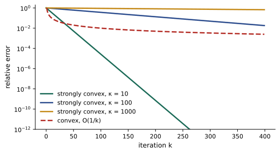
• Convex and \(L\)-smooth: \(f(\mathbf{w}_k) - f^* \le L\|\mathbf{w}_0 - \mathbf{w}^*\|^2/(2k)\). The error in function value falls as \(O(1/k)\): ten times more iterations give ten times smaller error.
• \(\mu\)-strongly convex and \(L\)-smooth: the function curves upward with curvature at least \(\mu > 0\) everywhere. Then \(\|\mathbf{w}_k - \mathbf{w}^*\|^2 \le (1 - \mu/L)^k\,\|\mathbf{w}_0 - \mathbf{w}^*\|^2\). The error shrinks by a constant factor each step: linear convergence, which on a logarithmic plot is a straight line.

The ratio \(\kappa = L/\mu\) is the condition number. Since \((1 - 1/\kappa)^k \approx e^{-k/\kappa}\), reaching relative accuracy \(\varepsilon\) takes about

iterations. A well-conditioned problem (\(\kappa\) near 1) converges in a handful of steps; an ill-conditioned one (\(\kappa = 10^4\)) needs tens of thousands.

Quadratics: the exact picture

A quadratic \(f(\mathbf{w}) = \tfrac12\mathbf{w}^\top A\mathbf{w} - \mathbf{b}^\top\mathbf{w}\) with symmetric positive definite \(A\) is the model problem, because near a minimum every smooth function looks like one. The gradient is \(A\mathbf{w} - \mathbf{b}\), and the error \(\mathbf{e}_k = \mathbf{w}_k - \mathbf{w}^*\) evolves as \(\mathbf{e}_{k+1} = (I - \eta A)\mathbf{e}_k\). In the eigenvector basis of \(A\), each component evolves independently:

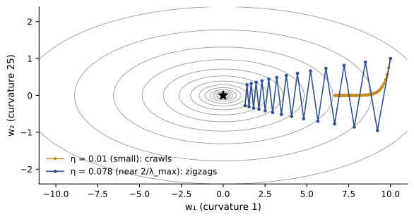
Component \(i\) shrinks if \(|1 - \eta\lambda_i| < 1\), that is, if \(\eta < 2/\lambda_i\). The step size must satisfy \(\eta < 2/\lambda_{\max}\) or the steepest direction diverges, while the flattest direction, with factor \(1 - \eta\lambda_{\min}\), converges slowest. The best fixed step, \(\eta = 2/(\lambda_{\min} + \lambda_{\max})\), balances the two and gives a contraction factor of \((\kappa - 1)/(\kappa + 1)\) per step.

import numpy as np

A = np.diag([1.0, 25.0])                  # condition number 25
w_star = np.zeros(2)
f = lambda w: 0.5 * w @ A @ w

def gd(eta, steps=60, w0=(10.0, 1.0)):
    w = np.array(w0)
    for _ in range(steps):
        w = w - eta * (A @ w)
    return f(w)

for eta in [0.01, 0.04, 2 / 26, 0.079, 0.081]:
    print(f"eta = {eta:.4f}:  f after 60 steps = {gd(eta):.3e}")

eta = 0.0100:  f after 60 steps = 1.497e+01
eta = 0.0400:  f after 60 steps = 3.728e-01
eta = 0.0769:  f after 60 steps = 4.211e-03
eta = 0.0790:  f after 60 steps = 6.016e-01
eta = 0.0810:  f after 60 steps = 2.420e+02

With \(\lambda_{\max} = 25\), the divergence threshold is \(2/25 = 0.08\). Small steps converge slowly because the flat direction (eigenvalue 1) barely moves; the optimal step \(2/26 \approx 0.077\) converges fastest; just below 0.08, the steep direction oscillates and decays very slowly; just above 0.08, it explodes.

Choosing the step size: line search

In practice \(L\) is unknown. Backtracking line search adapts the step at each iteration: start with a trial step \(t\) and shrink it by a factor \(\beta\) (often 0.5) until the Armijo sufficient-decrease condition holds:

with a small constant \(c\) such as \(10^{-4}\) or 0.5. Backtracking guarantees convergence at the same rates as the ideal fixed step, without knowing \(L\), at the cost of extra function evaluations. It is standard in classical optimization and in full-batch methods such as L-BFGS, but rarely used in deep learning, where each function evaluation on the full data set is expensive and stochastic gradients make the Armijo test unreliable; there, step sizes are tuned and scheduled instead (Lesson 3).

import numpy as np

rng = np.random.default_rng(0)
n, d = 500, 5
X = rng.normal(size=(n, d)) * np.array([1, 1, 1, 10, 0.1])   # badly scaled features
w_true = rng.normal(size=d)
y = (X @ w_true + rng.normal(size=n) > 0).astype(float)

def loss_grad(w):
    z = X @ w
    p = 1 / (1 + np.exp(-z))
    loss = np.mean(np.logaddexp(0, z) - y * z)
    return loss, X.T @ (p - y) / n

def gd_backtracking(w, iters=200, t0=1.0, beta=0.5, c=1e-4):
    evals = 0
    for _ in range(iters):
        f0, g = loss_grad(w); evals += 1
        t = t0
        while loss_grad(w - t * g)[0] > f0 - c * t * (g @ g):
            t *= beta; evals += 1
        w = w - t * g
    return w, loss_grad(w)[0], evals

w, f_end, evals = gd_backtracking(np.zeros(d))
print(f"final loss {f_end:.4f} after 200 iterations, {evals} function evaluations")

final loss 0.1102 after 200 iterations, 202 function evaluations

Conditioning and preconditioning

Many ill-conditioned problems become well-conditioned with a change of variables. In linear and logistic regression, the Hessian is built from \(X^\top X\) (weighted, in the logistic case), so features on very different scales produce eigenvalues on very different scales. Standardizing each feature to mean 0 and variance 1, as in AI-220, often reduces the condition number by orders of magnitude.

More generally, preconditioned gradient descent uses \(\mathbf{w}_{k+1} = \mathbf{w}_k - \eta P^{-1}\nabla f(\mathbf{w}_k)\) for a positive definite matrix \(P\) that approximates the Hessian. With \(P = \nabla^2 f\), this is Newton's method, which converges in one step on a quadratic. Diagonal preconditioners, which rescale each coordinate by an estimate of its curvature, are cheap, and the adaptive methods of Lesson 5 can be viewed as diagonal preconditioning learned from the gradients themselves.

import numpy as np

rng = np.random.default_rng(1)
X = rng.normal(size=(1000, 3)) * np.array([100.0, 1.0, 0.01])
Xs = (X - X.mean(0)) / X.std(0)
w_true = np.array([0.02, 1.0, 50.0])
y = X @ w_true + rng.normal(size=1000)

def iterations_to_converge(X, y, tol=1e-6, max_iter=200000):
    H = X.T @ X / len(y)
    eig = np.linalg.eigvalsh(H)
    eta = 1 / eig.max()
    w = np.zeros(X.shape[1])
    w_opt = np.linalg.lstsq(X, y, rcond=None)[0]
    for k in range(max_iter):
        if np.linalg.norm(w - w_opt) <= tol * np.linalg.norm(w_opt):
            return eig.max() / eig.min(), k
        w = w - eta * X.T @ (X @ w - y) / len(y)
    return eig.max() / eig.min(), None

for name, data in [("raw features", X), ("standardized", Xs)]:
    kappa, k = iterations_to_converge(data, y - y.mean() if name == "standardized" else y)
    result = f"{k} iterations" if k is not None else "not converged after 200,000 iterations"
    print(f"{name:13s} condition number {kappa:10.3e}   {result}")

raw features  condition number  9.706e+07   not converged after 200,000 iterations
standardized  condition number  1.152e+00   6 iterations

When to stop

Gradient descent never reaches the exact minimum, so a stopping rule is needed. Common criteria are a small gradient norm (\(\|\nabla f\| \le \epsilon\)), a small relative change in the loss or the parameters between iterations, or a fixed budget of iterations. In machine learning the real goal is generalization rather than the training loss, so training is often stopped when validation loss stops improving (early stopping), which also acts as a regularizer: for a quadratic loss started at zero, early-stopped gradient descent behaves much like ridge regression, with the number of steps playing the role of the inverse regularization strength.

How this course is organized

Lesson 1 studies gradient descent and Lesson 2 the convexity, smoothness and subgradients behind it. Lesson 3 adds the randomness of stochastic gradients, and Lesson 4 the curvature used by Newton and quasi-Newton methods. Lesson 5 covers momentum and adaptive methods such as Adam, and Lesson 6 the automatic differentiation that supplies every gradient. Lesson 7 treats constraints and convex optimization, and Lesson 8 the link between optimization and generalization. Lesson 9 examines the non-convex landscapes of deep networks, Lesson 10 hyperparameter optimization, and Lesson 11 derivative-free, evolutionary and discrete methods. Lesson 12 scales optimization to distributed and federated training and ends with a complete training project.