
ACCT-331 · Lesson 8 of 12 · 29 min
Audit sampling
An auditor of Fairhaven faces 1,180 wholesale customer accounts, 4,820 wholesale orders, 1.2 million retail transactions and tens of thousands of purchase invoices. Examining every one is impossible, so auditors examine some and draw conclusions about the rest. Audit sampling is the application of procedures to less than 100 per cent of a population in such a way that every sampling unit has a chance of selection, so that the auditor has a reasonable basis for conclusions about the whole population. This lesson explains when sampling applies, the risks it introduces, and the two main statistical methods: attribute sampling for tests of controls and monetary unit sampling for tests of details. It builds on the probability you learned in an introductory statistics course; the formulas are here, but the emphasis is on judgment.
When sampling applies
Not every selection is sampling. If the auditor examines all items above a certain amount, such as every customer balance over 500 thousand dollars, it is testing 100 per cent of that stratum, and there is no sampling risk for those items. If it selects specific items because they are unusual, such as the ten largest credit notes after year end, it is using judgment to target risk, but cannot project the results to the rest of the population. Sampling applies when the auditor wants to reach a conclusion about a whole population from a representative subset.
| Approach | What is selected | Can results be projected? |
|---|---|---|
| 100 per cent examination | Every item in the population or stratum | Not needed: everything is tested |
| Specific item selection | Key or high-value items, unusual items | No; the rest of the population needs other evidence |
| Audit sampling (statistical or non-statistical) | A sample in which every item has a chance of selection | Yes |
With data analytics, the auditor can increasingly test entire populations electronically for some attributes, such as whether every invoice has a matching shipping record. Sampling remains necessary when the procedure requires human judgment or physical evidence: sending confirmations, inspecting signatures, or counting inventory.
Sampling risk and non-sampling risk
Sampling risk is the risk that the auditor's conclusion based on a sample differs from the conclusion it would reach if it tested the whole population. It comes in two directions. The risk of incorrect acceptance (for tests of details) or the risk of assessing control risk too low (for tests of controls) is the risk of concluding things are fine when they are not; it affects audit effectiveness and is the serious one. The risk of incorrect rejection, or of assessing control risk too high, is the risk of concluding there is a problem when there is not; it affects efficiency, because the auditor does extra work that turns out to be unnecessary.
Non-sampling risk arises from factors unrelated to sampling: using an inappropriate procedure, misinterpreting evidence, or failing to recognize a misstatement or deviation. Examining every item would not remove non-sampling risk. Planning, supervision, review and the firm's quality management are the controls over it.
Statistical and non-statistical sampling
Statistical sampling uses random selection and probability theory to evaluate results, letting the auditor measure sampling risk. Non-statistical (judgmental) sampling relies on judgment to set sample sizes and evaluate results. Both are acceptable under auditing standards, and both require that the sample be representative and that the results be projected to the population. A non-statistical sample should be about as large as a well-designed statistical one with the same parameters; small judgmental samples, with no projection, are a common inspection finding.
CAS 530 governs audit sampling for audits under Canadian standards.
Selection methods include random selection, using random numbers to choose items; systematic selection, choosing every nth item from a random start; monetary unit selection, which gives larger items a proportionately higher chance; and haphazard selection, choosing items without a structured technique but without conscious bias, acceptable only for non-statistical samples. Block selection, choosing a group of consecutive items such as all December invoices, is rarely appropriate for sampling because a block is unlikely to represent the population.
Attribute sampling for tests of controls
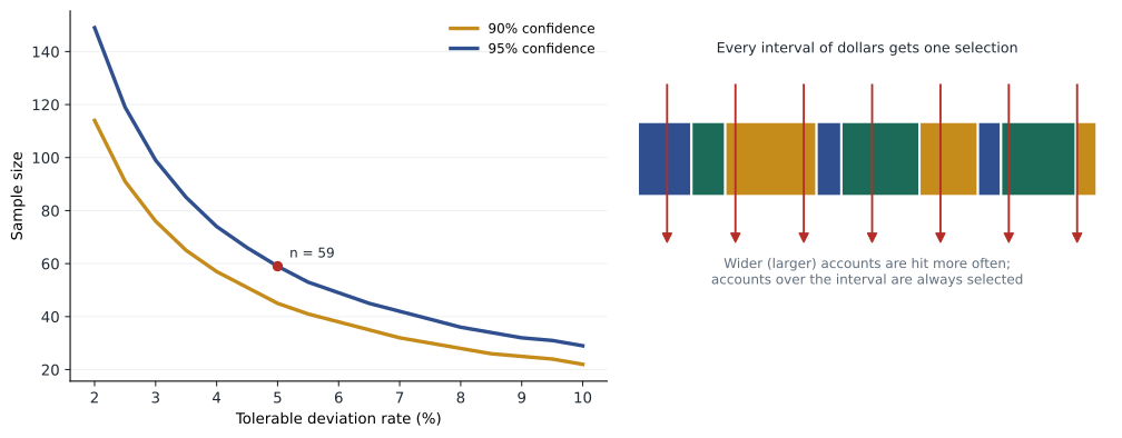
In a test of controls, each item either has the attribute (the control operated) or it does not (a deviation). Attribute sampling estimates the rate of deviations in the population. The auditor sets three parameters: the confidence level, usually 90 or 95 per cent; the tolerable deviation rate, typically 5 to 10 per cent depending on how much reliance is planned; and the expected deviation rate in the population, often zero. Population size has little effect on sample size once the population is more than a few thousand items, which surprises many students.
The sample size follows from the binomial distribution. With zero deviations expected, the auditor wants the smallest sample for which the probability of finding no deviations, if the true rate were at the tolerable level, is no more than one minus the confidence level.
Here, p_t is the tolerable deviation rate, n is the sample size and c is the confidence level. With a tolerable rate of 5 per cent and 95 per cent confidence, (0.95)^n must be at most 0.05, which first happens at n = 59. The program below computes sample sizes for several combinations, including samples that allow one deviation.
# Attribute sampling: sample size from the binomial distribution (zero expected deviations)
import math
def sample_size(confidence, tolerable, expected_dev=0):
    # smallest n such that P(at most expected_dev deviations | rate = tolerable) <= 1 - confidence
    n = 1
    while True:
        p = sum(math.comb(n, k) * tolerable**k * (1 - tolerable)**(n - k) for k in range(expected_dev + 1))
        if p <= 1 - confidence:
            return n
        n += 1
print(f"{'Confidence':<12}{'Tolerable':>10}{'Allowed devs':>14}{'n':>6}")
for conf in (0.90, 0.95):
    for tol in (0.05, 0.10):
        for k in (0, 1):
print(f"{conf:<12.0%}{tol:>10.0%}{k:>14}{sample_size(conf, tol, k):>6}")Confidence Tolerable Allowed devs n 90% 5% 0 45 90% 5% 1 77 90% 10% 0 22 90% 10% 1 38 95% 5% 0 59 95% 5% 1 93 95% 10% 0 29 95% 10% 1 46
Raising confidence or lowering the tolerable rate increases the sample; allowing for an expected deviation increases it further. The auditor evaluates results by computing the upper deviation limit, the highest rate the population could have at the chosen confidence given the deviations found, and comparing it with the tolerable rate. If the limit exceeds the tolerable rate, the control cannot be relied on as planned, as lesson 6 showed with Fairhaven's credit approval test. The auditor also considers the nature of each deviation: one deviation that suggests deliberate circumvention matters more than several clerical slips.
Monetary unit sampling for tests of details
For tests of details of balances, such as confirming receivables, the auditor wants to estimate the dollar amount of misstatement. Monetary unit sampling (MUS), also called probability-proportional-to-size sampling, treats each dollar in the population as a sampling unit. A customer account with a balance of 200,000 contains 200,000 units and is twenty times as likely to be selected as one with 10,000. This focuses testing on larger items, where overstatement matters most, and any item larger than the sampling interval is certain to be selected.
MUS is designed for testing overstatement. It is poor at detecting understatement, since an account recorded at zero or a small amount has little or no chance of selection, even if it should be large. For completeness of liabilities, auditors use other procedures, such as the search for unrecorded liabilities in lesson 10.
The sample size depends on the book value, the tolerable misstatement and a reliability factor based on the confidence level and the expected misstatement. With no expected misstatement and 95 per cent confidence, the reliability factor is 3.0 (derived from the Poisson distribution).
For Fairhaven's receivables of 21.4 million and tolerable misstatement of 410 thousand, the interval is about 136.7 thousand and the sample size about 157 selections. The auditor picks a random start within the first interval, then selects the account containing every 136,667th dollar. Some large accounts may be selected more than once; they are tested once.
Evaluating a monetary unit sample
When the auditor finds a misstatement, it calculates the tainting: the misstatement as a percentage of the book value of the item. For items smaller than the interval, the projected misstatement is the tainting multiplied by the interval, because the item represents the whole interval from which it was drawn. For items at or above the interval, the actual misstatement is used, without projection. The upper misstatement limit (UML) then adds three parts: basic precision (the reliability factor times the interval, the allowance for sampling risk even if no errors were found), the projected misstatements, and an incremental allowance for sampling risk on each misstatement, ranked by tainting.
# Monetary unit sampling of Fairhaven's wholesale receivables (dollars)
import math, random
random.seed(331)
customers = [round(random.lognormvariate(9.9, 1.1)) for _ in range(1_180)]
scale = 21_400_000 / sum(customers)                   # scale so the population equals the ledger balance
customers = [round(c * scale) for c in customers]
book = sum(customers)
tolerable = 410_000                                   # performance materiality
rf = 3.0                                              # reliability factor, 95% confidence, no expected misstatement
interval = tolerable / rf
n = math.ceil(book / interval)
print(f"Book value: {book:,}")
print(f"Sampling interval: {interval:,.0f}; sample size: {n}")

# systematic selection with a random start
start = random.randint(1, round(interval))
picks, cum, i, target = [], 0, 0, start
for idx, c in enumerate(customers):
    cum += c
    while cum >= target:
        if not picks or picks[-1] != idx:
            picks.append(idx)
        target += round(interval)
large = sum(1 for idx in picks if customers[idx] >= interval)
print(f"Customer accounts selected: {len(picks)}; accounts at or above the interval: {large}")

# two misstatements found by confirmation (book, audited)
errors = [(48_000, 36_000), (12_500, 0)]
print("Projected misstatement and upper misstatement limit")
basic = rf * interval
rows = []
for b, a in errors:
    taint = (b - a) / b
    proj = taint * (interval if b < interval else 0) + ((b - a) if b >= interval else 0)
    rows.append((taint, proj))
rows.sort(reverse=True)
factors = [1.75, 1.55]                                # incremental factors at 95% confidence for 1st and 2nd errors
upper = basic
for (taint, proj), f in zip(rows, factors):
    upper += proj * f
    print(f"  tainting {taint:.0%}: projected {proj:,.0f}, with allowance {proj * f:,.0f}")
total_proj = sum(p for _, p in rows)
print(f"Basic precision: {basic:,.0f}")
print(f"Total projected misstatement: {total_proj:,.0f}")
print(f"Upper misstatement limit: {upper:,.0f} vs tolerable {tolerable:,}")
print("Conclusion: balance may be materially misstated" if upper > tolerable else "Conclusion: accept the balance")Book value: 21,399,994 Sampling interval: 136,667; sample size: 157 Customer accounts selected: 149; accounts at or above the interval: 14 Projected misstatement and upper misstatement limit tainting 100%: projected 136,667, with allowance 239,167 tainting 25%: projected 34,167, with allowance 52,958 Basic precision: 410,000 Total projected misstatement: 170,833 Upper misstatement limit: 702,125 vs tolerable 410,000 Conclusion: balance may be materially misstated
Two misstatements were found. One customer's balance was overstated by 12,000 because a December shipment had been returned and the credit note was not recorded until January, a 25 per cent tainting. Another balance of 12,500 related to a customer who denied the debt entirely; investigation showed the invoice was recorded for goods that were never shipped, a 100 per cent tainting. The projected misstatement is about 171 thousand, but once the allowance for sampling risk is added, the upper misstatement limit is about 702 thousand, well above tolerable misstatement of 410 thousand.
The auditor cannot accept the balance as it stands. The options are to ask management to investigate the population for similar misstatements, such as reviewing all credit notes issued in January and all invoices without shipping documents, and correct them; to extend the sample; or to perform alternative procedures. If the misstatements cannot be resolved, they feed into the evaluation in lesson 11 and possibly into the opinion. The 100 per cent tainting deserves particular attention: an invoice for goods never shipped may be a fraud indicator, and the auditor must consider whether it is isolated or part of a pattern, given the presumed risk of fraud in revenue recognition.
| Component | Calculation | Amount |
|---|---|---|
| Basic precision | 3.0 × 136,667 | 410,000 |
| First misstatement (100% tainting) | 1.00 × 136,667 × 1.75 | 239,167 |
| Second misstatement (25% tainting) | 0.25 × 136,667 × 1.55 | 52,958 |
| Upper misstatement limit | Sum | 702,125 |
| Tolerable misstatement | Performance materiality | 410,000 |
Classical variables sampling
An alternative to MUS for tests of details is classical variables sampling, which uses the normal distribution. Methods include mean-per-unit estimation, difference estimation and ratio estimation. Classical methods handle understatements and zero balances better than MUS and can be more efficient when many misstatements are expected, but they require larger samples when misstatements are rare and are more complex to apply. In practice, MUS dominates tests of receivables and inventory pricing, while classical methods appear in specialized settings such as LIFO inventory pools or large populations with frequent small differences.
Worked problem
Choosing a sampling method
For each test, choose attribute sampling, MUS, or neither: (a) testing whether purchase invoices were approved; (b) confirming receivables for overstatement; (c) searching for unrecorded liabilities.
Show solution
- (a) A yes/no control test: attribute sampling.
- (b) Dollar overstatement in a balance: MUS.
- (c) Understatement: MUS gives little chance of selecting omitted items, so use a targeted search of subsequent payments instead.
Answer: (a) attribute sampling, (b) MUS, (c) a targeted procedure rather than MUS.
Worked problem
Projecting a misstatement
In an MUS sample with an interval of 136,667, an account with a book value of 40,000 is found to be overstated by 10,000. What is the projected misstatement?
Show solution
- Tainting = 10,000 / 40,000 = 25 per cent.
- The item is smaller than the interval, so project over the interval.
- Projected = 0.25 × 136,667 = 34,167.
Answer: About 34,167.
Common mistakes
MistakeTreating a selection of the largest items as a sample.
InsteadSelecting specific items is not sampling; results cannot be projected to the rest.
MistakeAssuming population size drives the sample size.
InsteadFor large populations, confidence and tolerable rates drive sample size; population size has little effect.
MistakeUsing MUS to test for understatement.
InsteadUnderstated or omitted items have little chance of selection; use other procedures.
MistakeEvaluating a sample only by its error rate.
InsteadAdd an allowance for sampling risk: compare the upper limit, not the sample rate, with the tolerable amount.
MistakeIgnoring the nature of a deviation or misstatement.
InsteadA deliberate or fraudulent item matters more than its size suggests.
Summary and key terms
- Sampling applies when every unit has a chance of selection and results are projected to the population.
- Incorrect acceptance (effectiveness) is the serious sampling risk; incorrect rejection affects efficiency.
- Statistical and non-statistical sampling are both acceptable, but non-statistical samples should be similar in size.
- Attribute sampling estimates deviation rates: 59 items for 95 per cent confidence and a 5 per cent tolerable rate with no expected deviations.
- MUS treats each dollar as a unit, favours large items and is designed to detect overstatement.
- The upper misstatement limit combines basic precision, projected misstatement and incremental allowances.
- At Fairhaven, the receivables UML exceeds tolerable misstatement, so further work is needed.
- Audit sampling
- Applying procedures to less than 100 per cent of a population so that every unit has a chance of selection.
- Sampling risk
- The risk that a conclusion based on a sample differs from that based on the whole population.
- Non-sampling risk
- The risk of a wrong conclusion for reasons unrelated to sampling.
- Risk of incorrect acceptance
- The risk of concluding a balance is not materially misstated when it is.
- Attribute sampling
- Sampling to estimate the rate of occurrence of a characteristic, such as a control deviation.
- Monetary unit sampling
- Sampling in which each dollar is a sampling unit, so larger items are more likely to be chosen.
- Sampling interval
- The number of dollars between selections in monetary unit sampling.
- Tainting
- A misstatement expressed as a percentage of the item's book value.
- Upper misstatement limit
- The maximum misstatement in the population at a given confidence level.
- Reliability factor
- A factor based on confidence and expected misstatement, used to set MUS sample size.
Practice problems
Work each problem on paper first, then reveal the answer to check.
Why is selecting all accounts over 500 thousand not audit sampling?
Show answer
Every item in that stratum is tested, so nothing is projected.
Which sampling risk affects audit effectiveness?
Show answer
The risk of incorrect acceptance (or assessing control risk too low).
Rerun the attribute program. What sample size gives 90 per cent confidence and a 10 per cent tolerable rate with zero expected deviations?
Show answer
22.
Show that 59 is the right size for 95 per cent and 5 per cent.
Show answer
0.95 to the power 59 is about 0.048, at most 0.05; 0.95 to the power 58 is about 0.051.
With a tolerable misstatement of 300,000 and RF 3.0, what is the MUS interval for 21.4 million of receivables, and the sample size?
Show answer
Interval 100,000; sample about 214.
Why is MUS poor at detecting understatement?
Show answer
Small or omitted items have little or no chance of selection.
An item of 200,000 is selected with an interval of 136,667 and is overstated by 20,000. What misstatement is used?
Show answer
20,000, the actual misstatement, because the item exceeds the interval.
Rerun the MUS program without the 100 per cent tainting. Is the balance acceptable?
Show answer
UML is about 410,000 + 0.25 × 136,667 × 1.75, roughly 470,000, still above 410,000.
When is block selection appropriate for sampling?
Show answer
Rarely, because a block is unlikely to represent the population.
Name one advantage of classical variables sampling over MUS.
Show answer
It handles understatements and zero balances better.
Lesson quiz · 5 questions
Score 60% or more to complete this lesson.
Create a free account to save your progress, take quizzes and earn a certificate.