
ROB-340 · Lesson 9 of 12 · 30 min
Lidar SLAM in practice
Lidar is the workhorse sensor for SLAM on industrial mobile robots, autonomous vehicles and survey systems. It measures range directly, with centimeter accuracy, independent of lighting, and modern 3-D lidars return hundreds of thousands of points per second. A practical lidar SLAM system combines the pieces from earlier lessons: a front end that estimates motion by registering scans and proposes loop closures, and a graph-based back end that optimizes the trajectory. This lesson covers scan registration in depth (ICP and its variants, NDT and correlative matching), degeneracy, the structure of widely used open-source systems (Cartographer, slam_toolbox, and the LOAM and LIO-SAM family for 3-D), and how lidar is fused with inertial measurements. Specific packages and versions are described as they stood at the time of writing; the field moves quickly.
Scan registration with ICP
Scan registration finds the rigid transform (a rotation R and translation t) that best aligns a new scan with a reference, which may be the previous scan, a recent window of scans, or the map. Iterative closest point (ICP) alternates two steps: for each point in the new scan, find the closest point in the reference using a k-d tree; then compute the transform that minimizes the sum of squared distances between the pairs. For point-to-point pairs, the second step has a closed-form solution: subtract the centroids, form the 2 × 2 or 3 × 3 cross-covariance matrix, take its singular value decomposition \( W = U\Sigma V^{\mathsf{T}} \), and set \( R = VU^{\mathsf{T}} \) (with a sign correction if needed) and t from the centroids. The two steps repeat until the change is small.
Point-to-point ICP converges slowly on flat surfaces, because points slide along a wall without any cost. Point-to-plane ICP (Chen and Medioni, 1991) minimizes the distance from each point to the tangent plane (or line, in 2-D) at its match, \( \sum ((R\mathbf{p}_i + \mathbf{t} - \mathbf{q}_i)\cdot\mathbf{n}_i)^2 \), which converges in far fewer iterations in structured environments. Generalized ICP (Segal, Haehnel and Thrun, 2009) models both scans as locally planar Gaussians and is a common default in 3-D. Every ICP variant needs a reasonable initial guess, usually from odometry or an IMU, because it converges only to the nearest local minimum, and it needs outlier rejection (discarding pairs farther apart than a threshold) to cope with dynamic objects and partial overlap.
Worked problem
One closed-form ICP alignment step
Three matched point pairs in 2-D: scan points (0, 0), (2, 0), (0, 1) correspond to reference points (1, 1), (1, 3), (0, 1). Find the rotation and translation that aligns the scan to the reference.
Show solution
- Scan centroid: (0.667, 0.333); reference centroid: (0.667, 1.667).
- Centered scan: (−0.667, −0.333), (1.333, −0.333), (−0.667, 0.667). Centered reference: (0.333, −0.667), (0.333, 1.333), (−0.667, −0.667).
- Each centered reference point equals the centered scan point rotated by +90°: (x, y) maps to (−y, x). So R is a 90° rotation.
- t = reference centroid − R × scan centroid = (0.667, 1.667) − (−0.333, 0.667) = (1.0, 1.0).
Answer: R is a rotation by +90° and t = (1, 1). The SVD formula gives the same answer; with noisy points it gives the least-squares best fit.
import numpy as np
rng = np.random.default_rng(8)
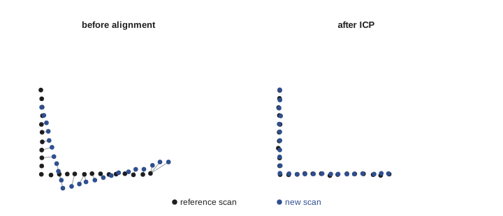
# an L-shaped corner seen in two scans; the second robot pose is moved and turned
wall = np.vstack([np.column_stack([np.linspace(0, 4, 80), np.zeros(80)]),
                  np.column_stack([np.zeros(60), np.linspace(0, 3, 60)])])
th, t_true = np.radians(8), np.array([0.30, -0.20])
R_true = np.array([[np.cos(th), -np.sin(th)], [np.sin(th), np.cos(th)]])
ref = wall + rng.normal(0, 0.01, wall.shape)
scan = (wall - t_true) @ R_true + rng.normal(0, 0.01, wall.shape)    # same walls seen from moved pose
R, t = np.eye(2), np.zeros(2)
for it in range(30):
    moved = scan @ R.T + t
    d = np.linalg.norm(moved[:, None, :] - ref[None, :, :], axis=2)
    j = d.argmin(1); keep = d[np.arange(len(moved)), j] < 0.5         # reject far pairs
    P, Qp = moved[keep], ref[j[keep]]
    pc, qc = P.mean(0), Qp.mean(0)
    U, S, Vt = np.linalg.svd((P - pc).T @ (Qp - qc))
    dR = Vt.T @ U.T
    if np.linalg.det(dR) < 0: Vt[1] *= -1; dR = Vt.T @ U.T
    dt = qc - dR @ pc
    R, t = dR @ R, dR @ t + dt
    if np.abs(dt).max() < 1e-5 and abs(np.arctan2(dR[1, 0], dR[0, 0])) < 1e-6: break
print("ICP converged in %d iterations" % (it + 1))
print("estimated rotation %.2f deg (true %.2f), translation (%.3f, %.3f) (true %.3f, %.3f)" %
(np.degrees(np.arctan2(R[1, 0], R[0, 0])), np.degrees(th), *t, *t_true))ICP converged in 21 iterations estimated rotation 8.00 deg (true 8.00), translation (0.301, -0.201) (true 0.300, -0.200)
NDT and correlative scan matching
The normal distributions transform (NDT, Biber and Strasser for 2-D in 2003, Magnusson for 3-D in 2009) avoids explicit nearest-neighbor pairing. It divides the reference into cells and fits a Gaussian (mean and covariance) to the points in each cell; the match score of a candidate pose is the sum of the Gaussian likelihoods of the transformed scan points. This score is smooth and differentiable, so Newton's method converges quickly, and the map is compact. NDT is widely used for localizing autonomous vehicles in prebuilt 3-D maps.
Correlative scan matching (Olson, 2009) evaluates the match score exhaustively over a grid of candidate poses within a search window, using a precomputed likelihood grid and a coarse-to-fine strategy to make this fast. It is robust to poor initial guesses, finds the global best match within the window, and naturally yields a covariance from the shape of the score around its peak. Cartographer uses a branch-and-bound version for loop closure, and Karto (the core of slam_toolbox) uses correlative matching for both odometry and loop closure.
| Method | Matching principle | Initial guess needed | Notes |
|---|---|---|---|
| ICP point-to-point | Nearest neighbor pairs, closed-form step | Good | Simple; slow on planes |
| ICP point-to-plane | Point to tangent plane distance | Good | Fast convergence in buildings |
| Generalized ICP | Plane-to-plane Gaussian model | Good | Common 3-D default |
| NDT | Gaussians per cell, smooth score | Moderate | Compact maps; vehicle localization |
| Correlative | Exhaustive score over a pose grid | Weak (within window) | Robust; gives covariance; loop closure |
Degeneracy
Registration can be geometrically ill-posed. In a long, straight corridor with plain walls, every scan looks the same no matter where along the corridor it is taken, so the motion along the corridor is unobservable; in an open field with flat ground, horizontal motion is unobservable; in a tunnel, motion along the axis is. The matcher still returns an answer, but its error in the degenerate direction can be large, and a SLAM system that trusts it will stretch or shrink the map. Degeneracy can be detected from the Hessian (or information matrix) of the registration cost: an eigenvalue much smaller than the others means a direction in which the cost is nearly flat. Zhang, Kaess and Singh (2016) proposed solving the registration only in the well-constrained directions and leaving the others to the motion prior. Practical remedies are fusing an IMU and wheel odometry, adding reflectors or other features, and down-weighting lidar odometry when degeneracy is detected.
Worked problem
Detecting a degenerate direction
The 2-D translational part of a point-to-line registration Hessian in a corridor is \( \begin{bmatrix} 2 & 0 \\ 0 & 1800 \end{bmatrix} \) (in arbitrary units), with x along the corridor. What are the eigenvalues and condition number, and what does this mean?
Show solution
- The matrix is diagonal, so the eigenvalues are 2 (along x) and 1800 (along y).
- Condition number: \( 1800/2 = 900 \).
- Cost changes 900 times more slowly along the corridor than across it.
Answer: Motion along the corridor is nearly unobservable from the scans. The system should rely on wheel odometry or an IMU in that direction rather than trusting the lidar estimate.
import numpy as np
# Information (Hessian) of point-to-line registration: sum of n n^T over points
def info(normals):
    return sum(np.outer(n, n) for n in normals)
corridor = [np.array([0.0, 1.0])] * 200 + [np.array([0.0, -1.0])] * 200   # two long walls
room = corridor[:200] + [np.array([1.0, 0.0])] * 150 + [np.array([-1.0, 0.0])] * 150
for name, nrm in [("corridor", corridor), ("room", room)]:
    ev = np.linalg.eigvalsh(info(nrm))
    print("%-8s eigenvalues %s -> condition %s" % (name, np.round(ev, 1),
"infinite (degenerate)" if ev[0] < 1e-9 else round(ev[1] / ev[0], 2)))corridor eigenvalues [ 0. 400.] -> condition infinite (degenerate) room eigenvalues [200. 300.] -> condition 1.5
Open-source 2-D lidar SLAM
Cartographer, released by Google in 2016 (Hess, Kohler, Rapp and Andor), builds small local submaps by matching scans to the current submap with a Ceres-based scan matcher, and runs a global pose-graph optimization in the background that adds loop closures found by fast branch-and-bound correlative matching against older submaps. It supports 2-D and 3-D lidars and IMUs and produces high-quality maps of large buildings; its development slowed after Google archived the project, though community forks remained in use at the time of writing.
slam_toolbox, by Steve Macenski, is the default 2-D SLAM package in ROS 2 Nav2 at the time of writing. It builds on the Karto scan matcher and graph optimizer and adds the features needed for deployment: lifelong mapping (continuing to update a saved map on later runs while removing outdated nodes), serialization and loading of the pose graph rather than just a grid image, interactive manual loop closure and graph editing in RViz, multi-session mapping, and a pure localization mode that matches scans to the saved graph instead of running AMCL.
# slam_toolbox (ROS 2) - excerpt of a mapping configuration
slam_toolbox:
  ros__parameters:
    mode: mapping                    # or localization
    resolution: 0.05
    max_laser_range: 12.0
    minimum_travel_distance: 0.3     # add a node after 0.3 m ...
    minimum_travel_heading: 0.3      # ... or 0.3 rad of rotation
    do_loop_closing: true
    loop_search_maximum_distance: 4.0
    loop_match_minimum_response_fine: 0.45
    map_update_interval: 5.0
3-D lidar and lidar-inertial SLAM
Spinning 3-D lidars introduce a complication: the sensor takes about 100 ms to sweep 360°, during which a moving robot travels and turns, so the points of one scan are measured from different poses. Without correction, walls appear bent and doubled. Deskewing (motion compensation) uses odometry or an IMU to transform every point to a common time. LOAM (lidar odometry and mapping, Zhang and Singh, 2014) extracted edge and planar feature points by local curvature and registered them at two rates, a fast odometry step and a slower mapping step, and it topped the KITTI odometry benchmark for years. LeGO-LOAM (2018) added ground segmentation for vehicles; LIO-SAM (Shan and colleagues, 2020) placed lidar odometry, IMU preintegration, GPS and loop closures in a single factor graph solved with iSAM2. FAST-LIO and FAST-LIO2 (Xu and Zhang, 2021–2022) use an iterated error-state Kalman filter with an incremental k-d tree and registered raw points directly, achieving very fast lidar-inertial odometry on embedded computers. KISS-ICP (Vizzo and colleagues, 2023) showed that a carefully engineered point-to-point ICP with adaptive thresholds can be competitive with far more complex pipelines.
Worked problem
How much does motion distort a scan?
A vehicle moves at 15 m/s with a 10 Hz spinning lidar. How far does it travel during one sweep? If it also yaws at 30° per second, how much does its heading change?
Show solution
- Sweep time: 0.1 s.
- Distance: \( 15 \times 0.1 = 1.5 \) m.
- Heading change: \( 30 \times 0.1 = 3^{\circ} \).
Answer: 1.5 m and 3° within one scan. A wall 20 m away would be smeared by about \( 20 \times 0.052 = 1 \) m from the rotation alone, so deskewing with an IMU is essential for 3-D lidar SLAM on moving vehicles.
Tuning and validating a lidar SLAM system
The parameters that matter most are the scan registration thresholds (maximum correspondence distance, number of iterations), the node spacing (how far the robot moves before a new pose is added), the loop closure search radius and acceptance threshold, and the noise models of the constraints. Mapping runs should be planned: drive slowly, revisit places to create loop closures early and often, avoid long excursions into featureless areas, and give the system a few seconds at the start to initialize. Validate maps against ground truth where possible (surveyed points, a total station, or a known building plan) and compute the trajectory metrics described in lesson 11.
Common mistakes
MistakeRunning ICP without an initial guess from odometry
InsteadSeed registration with odometry or an IMU so it converges to the right minimum.
MistakeAccepting every nearest-neighbor pair
InsteadReject pairs beyond a distance threshold to handle dynamic objects and partial overlap.
MistakeTrusting lidar odometry in long featureless corridors
InsteadCheck registration degeneracy and rely on other sensors in weak directions.
MistakeUsing raw 3-D lidar scans on a moving vehicle
InsteadDeskew points to a common time using odometry or an IMU.
MistakeMapping in one long pass with no revisits
InsteadPlan routes that close loops early and often.
Summary and key terms
- Lidar SLAM combines scan-registration front ends with graph-based back ends.
- ICP alternates nearest-neighbor pairing with a closed-form (SVD) transform; point-to-plane and GICP converge faster.
- NDT matches scans to per-cell Gaussians; correlative matching searches a pose grid and gives a covariance.
- Degenerate geometry, such as long corridors, leaves directions unobservable; the Hessian's small eigenvalues reveal it.
- Cartographer and slam_toolbox build submaps or pose graphs with correlative loop closure for 2-D lidar.
- 3-D lidar needs deskewing; LOAM, LIO-SAM, FAST-LIO and KISS-ICP are representative systems.
- Planned mapping routes with frequent loop closures and validation against ground truth give the best maps.
- Scan registration
- Finding the transform that aligns one scan with another or with a map.
- ICP
- Iterative closest point, alternating correspondence search and transform estimation.
- Point-to-plane ICP
- ICP minimizing distances from points to tangent planes.
- NDT
- Normal distributions transform, matching points to per-cell Gaussians.
- Correlative scan matching
- Exhaustive scoring of candidate poses over a search window.
- Degeneracy
- Geometry in which some motion directions are unobservable from the scans.
- Deskewing
- Correcting points of a sweeping lidar for motion during the sweep.
- Submap
- A small local map built from consecutive scans, later aligned globally.
- Lifelong mapping
- Continuing to update a saved map across many sessions.
- Lidar-inertial odometry
- Motion estimation fusing lidar registration with an IMU.
Practice problems
Work each problem on paper first, then reveal the answer to check.
What are the two alternating steps of ICP?
Show answer
Find nearest-neighbor correspondences; compute the best rigid transform.
How is the point-to-point ICP rotation computed?
Show answer
From the SVD of the cross-covariance of centered point sets.
Why does point-to-plane ICP converge faster in buildings?
Show answer
Points are not penalized for sliding along walls; distances are measured along normals.
What does NDT store in each cell?
Show answer
A Gaussian (mean and covariance) of the points.
Name an advantage of correlative scan matching.
Show answer
Robust to poor initial guesses, and it gives a covariance.
Hessian eigenvalues 5 and 2,000: condition number?
Show answer
400.
A vehicle at 20 m/s with a 10 Hz lidar travels how far per sweep?
Show answer
2 m.
What does slam_toolbox's localization mode match against?
Show answer
The saved pose graph.
Name a lidar-inertial SLAM system.
Show answer
LIO-SAM or FAST-LIO.
Why plan mapping routes with revisits?
Show answer
To create loop closures early and often.
Lesson quiz · 5 questions
Score 60% or more to complete this lesson.
Create a free account to save your progress, take quizzes and earn a certificate.