
ROB-340 · Lesson 10 of 12 · 29 min
Visual and visual-inertial SLAM
Cameras are cheap, light, low-power and information-rich, which makes visual SLAM attractive for drones, consumer robots, phones, headsets and cars. A camera sees texture and appearance that a lidar cannot, which helps place recognition, but it does not measure depth directly (unless it is a stereo or RGB-D camera), it struggles in darkness and on blank surfaces, and a single camera cannot observe scale. Adding an inertial measurement unit fixes much of this: the IMU provides metric scale, gravity direction and smooth motion over short gaps, while the camera bounds the IMU's drift. Visual-inertial odometry and SLAM now run on billions of phones for augmented reality. ROB-330 lesson 7 covered visual odometry and bundle adjustment; this lesson builds complete visual and visual-inertial SLAM systems on that foundation.
The structure of a visual SLAM system
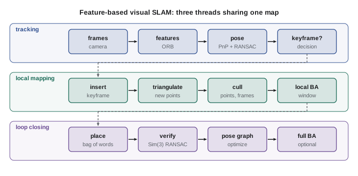
A feature-based visual SLAM system typically runs three threads. Tracking estimates the camera pose for every frame by matching features to the local map and solving perspective-n-point with RANSAC, then refining the pose by minimizing reprojection error. Local mapping decides when to insert a new keyframe, triangulates new map points from matches between keyframes, culls redundant points and keyframes, and runs local bundle adjustment over a window of recent keyframes and the points they observe. Loop closing searches for revisited places, verifies candidates geometrically, and when a loop is accepted, corrects the drift with a pose-graph optimization followed, optionally, by full bundle adjustment. This architecture was introduced by PTAM (Klein and Murray, 2007), which first split tracking and mapping into parallel threads, and refined by ORB-SLAM.
ORB-SLAM and keyframe-based maps
ORB-SLAM (Mur-Artal, Montiel and Tardós, 2015) became the reference feature-based visual SLAM system. It uses ORB features (fast binary descriptors) for everything: tracking, mapping, relocalization and loop closure. Its map consists of keyframes, map points with descriptors, and a covisibility graph linking keyframes that see the same points, which defines the local window for tracking and bundle adjustment. An essential graph, a sparser subset of covisibility edges plus a spanning tree and loop edges, is used for fast pose-graph optimization at loop closure. ORB-SLAM2 (2017) added stereo and RGB-D cameras, and ORB-SLAM3 (Campos and colleagues, 2021) added tightly coupled visual-inertial operation and multi-map management (the Atlas), which lets the system start a new map when tracking is lost and merge it with an old one when a common place is recognized.
Keyframe selection is important for both efficiency and accuracy. Inserting every frame would make bundle adjustment slow and the map redundant; inserting too few would lose tracking during fast motion. Typical criteria are a minimum number of frames since the last keyframe, a drop in the fraction of map points tracked (for example below 90 % of the reference keyframe's), and sufficient parallax for triangulation. Redundant keyframes, whose points are mostly seen by other keyframes, are culled later.
Worked problem
Keyframe budget for a long run
A visual SLAM system on a robot moving at 1 m/s inserts a keyframe on average every 0.4 m. Each keyframe stores 1,000 ORB features (32-byte descriptor plus 16 bytes of keypoint data) and the map adds about 150 new map points per keyframe at 60 bytes each. How much memory does a 2 km run need?
Show solution
- Keyframes: \( 2000/0.4 = 5000 \).
- Per keyframe: \( 1000 \times 48 = 48 \) kB of features and \( 150 \times 60 = 9 \) kB of points, about 57 kB.
- Total: \( 5000 \times 57 \) kB, about 285 MB.
Answer: About 285 MB, manageable, but growing linearly with distance. Keyframe culling and map management matter for robots that operate for hours every day.
Direct and dense methods
Feature-based methods throw away most of the image. Direct methods instead minimize photometric error, the difference in pixel brightness between images warped by the estimated motion and depth, using all pixels with sufficient gradient. LSD-SLAM (Engel, Schöps and Cremers, 2014) built semi-dense maps with direct alignment, and DSO (direct sparse odometry, 2018) jointly optimized poses, sparse depths and a photometric camera model including exposure times and lens vignetting. Direct methods track well in low-texture scenes with edges and gradients, but they require careful photometric calibration and are sensitive to rolling-shutter effects and lighting changes. Dense RGB-D SLAM, such as KinectFusion and ElasticFusion, fuses depth images into detailed surface models for small and medium-scale scenes. Learned methods, such as DROID-SLAM (Teed and Deng, 2021) and SLAM systems built on neural radiance fields and Gaussian splatting, were active research areas at the time of writing.
Place recognition with bags of visual words
Loop closure in visual SLAM relies on fast place recognition among thousands of keyframes. The bag-of-visual-words approach, borrowed from text retrieval, quantizes descriptors into a vocabulary of visual words using a tree built offline by hierarchical k-means on a large image set. Each image becomes a sparse histogram of word counts, weighted by term frequency-inverse document frequency (tf-idf) so that common words count less, and two images are compared by a similarity score between their histograms. An inverted index (for each word, the list of images containing it) makes retrieval fast. DBoW2 (Gálvez-López and Tardós, 2012) is the library used by ORB-SLAM. Candidates retrieved by appearance are then checked for consistency with neighboring keyframes and verified geometrically, by computing a relative pose (a similarity transform for monocular systems, to correct scale drift) with RANSAC.
import numpy as np
rng = np.random.default_rng(6)
V = 500                                     # vocabulary size (visual words)
def image(place, n=300):                    # each place has a typical word distribution
    p = np.ones(V); p[place * 40:(place + 1) * 40] += 25       # distinctive words
    p[:20] += 60                                                  # words common everywhere
    return np.bincount(rng.choice(V, n, p=p / p.sum()), minlength=V)
db = np.array([image(k) for k in range(10)])   # keyframes from 10 different places
idf = np.log(len(db) / np.maximum(1, (db > 0).sum(0)))
def vec(h):
    v = (h / h.sum()) * idf
    return v / np.linalg.norm(v)
D = np.array([vec(h) for h in db])
query = vec(image(6))                           # robot revisits place 6
scores = D @ query
best = np.argsort(scores)[::-1][:3]
print("top matches (place, score):", [(int(b), round(float(scores[b]), 3)) for b in best])
raw = db / np.linalg.norm(db, axis=1, keepdims=True)
qraw = image(6); qraw = qraw / np.linalg.norm(qraw)
print("without idf weighting, best score margin: %.3f" % (np.sort(raw @ qraw)[-1] - np.sort(raw @ qraw)[-2]))
print("with idf weighting, best score margin: %.3f" % (np.sort(scores)[-1] - np.sort(scores)[-2]))top matches (place, score): [(6, 0.656), (5, 0.064), (7, 0.052)] without idf weighting, best score margin: 0.077 with idf weighting, best score margin: 0.592
Scale, and why monocular SLAM drifts in scale
A single camera cannot distinguish a large scene far away from a small scene close up, so monocular SLAM reconstructs the world only up to an unknown scale, and that scale drifts slowly along the trajectory as small errors accumulate. At a loop closure, the relative transform between the two ends must therefore be estimated as a similarity transform, Sim(3), with seven degrees of freedom (rotation, translation and scale), and the pose-graph optimization distributes the scale correction around the loop. Strasdat, Montiel and Davison showed this in 2010. Stereo and RGB-D cameras measure metric depth directly and avoid scale drift; so does an IMU.
Worked problem
Correcting scale drift at a loop closure
A monocular SLAM system completes a loop. Measured by the loop-closure similarity transform, the map at the end of the loop is at scale 0.94 relative to the start. If the drift is spread evenly over 200 keyframes, what scale correction factor is applied per keyframe?
Show solution
- Total correction needed: \( 1/0.94 = 1.0638 \).
- Per keyframe, spread geometrically: \( 1.0638^{1/200} = e^{\ln(1.0638)/200} = e^{0.0619/200} \).
- \( e^{0.000309} \approx 1.00031 \).
Answer: About 1.0003 per keyframe, a 0.03 % scale adjustment each, compounding to the 6.4 % total. Spreading the correction keeps the map locally consistent.
Visual-inertial odometry and SLAM
An IMU measures angular velocity and specific force (acceleration minus gravity) at hundreds of hertz. Integrated between camera frames, it predicts motion, makes scale and the gravity direction observable, and bridges short visual failures such as motion blur or a blank wall. IMU measurements are corrupted by biases that drift slowly, so the biases are estimated as part of the state. Visual-inertial systems are either loosely coupled, fusing a separate visual pose estimate with the IMU in a filter, or tightly coupled, putting raw feature measurements and IMU measurements into one estimator, which is more accurate and is standard today.
Because IMU data arrive far faster than images, optimization-based systems use IMU preintegration (Lupton and Sukkarieh, 2012; Forster, Carlone, Dellaert and Scaramuzza, 2017): the many IMU samples between two keyframes are combined into a single relative-motion factor, a change in rotation, velocity and position, that does not need to be recomputed when the keyframe poses change, with first-order corrections for changes in the bias estimates. Representative systems include the MSCKF filter (lesson 6), OKVIS (Leutenegger and colleagues, 2015), VINS-Mono and VINS-Fusion (Qin, Li and Shen, 2018), Basalt, and ORB-SLAM3's visual-inertial mode. Phone and headset tracking (ARCore, ARKit and similar) is built on the same principles.
Worked problem
How quickly does an IMU alone drift?
An uncorrected accelerometer bias of 0.02 m/s² (a typical consumer MEMS value after rough calibration) is double-integrated for 10 s while the camera sees nothing. What position error results? What about 1 s?
Show solution
- Position error from constant bias: \( \tfrac{1}{2} b t^2 \).
- At 10 s: \( 0.5 \times 0.02 \times 100 = 1.0 \) m.
- At 1 s: \( 0.5 \times 0.02 \times 1 = 0.01 \) m.
Answer: About 1 m after 10 s but only 1 cm after 1 s. An IMU easily bridges a second of visual dropout, but not long ones, which is why visual updates and bias estimation are both essential.
| System | Sensors | Approach | Notable features |
|---|---|---|---|
| ORB-SLAM3 | Mono, stereo, RGB-D, with or without IMU | Feature-based, keyframes, BA | Multi-map Atlas, robust relocalization |
| VINS-Mono / VINS-Fusion | Mono or stereo camera plus IMU (and GPS) | Tightly coupled sliding-window optimization | Online extrinsic and time-offset calibration |
| OKVIS | Stereo or mono plus IMU | Keyframe sliding-window optimization | Early tightly coupled reference system |
| MSCKF-based | Camera plus IMU | Filter with window of camera poses | Low computation, common on embedded hardware |
| DSO | Monocular | Direct photometric optimization | Works on low-texture scenes with gradients |
Practical issues
Visual SLAM depends on details that are easy to get wrong. Camera intrinsics and distortion must be calibrated (ROB-330 lesson 3), and for visual-inertial systems so must the camera-IMU extrinsic transform and the time offset between the sensors, using tools such as Kalibr; a few milliseconds of time offset at high rotation rates causes large errors. Global-shutter cameras avoid rolling-shutter distortion during fast motion. Auto-exposure changes break direct methods unless exposure is known. Dynamic objects, such as people and vehicles, should be rejected as outliers or masked with a detector. Lighting changes between day and night, and seasonal changes outdoors, defeat appearance-based place recognition, which motivates learned descriptors and multi-session maps. And because errors accumulate silently, a deployed system should monitor its health: the number of tracked features, the inlier ratio, the reprojection error and the IMU bias estimates.
Common mistakes
MistakeRunning visual-inertial SLAM without calibrating the camera-IMU time offset
InsteadCalibrate extrinsics and time offset, or estimate them online.
MistakeClosing monocular loops with a rigid transform
InsteadUse a similarity transform, so scale drift can be corrected.
MistakeInserting a keyframe for every frame
InsteadSelect keyframes by tracking quality and parallax, and cull redundant ones.
MistakeTrusting appearance matches without geometric verification
InsteadVerify candidates with a RANSAC relative-pose estimate and consistency checks.
MistakeUsing a rolling-shutter camera for fast motion without modeling it
InsteadPrefer global shutter or model the rolling shutter.
Summary and key terms
- Visual SLAM systems run tracking, local mapping and loop closing over a shared keyframe map.
- ORB-SLAM uses ORB features throughout, with covisibility and essential graphs for local and global optimization.
- Direct methods minimize photometric error and need photometric calibration; dense methods fuse depth into surfaces.
- Bag-of-visual-words with tf-idf and an inverted index gives fast place recognition, followed by geometric verification.
- Monocular SLAM drifts in scale, so loop closures use similarity transforms; stereo, RGB-D and IMUs provide scale.
- Tightly coupled visual-inertial systems estimate motion, scale, gravity and IMU biases, using IMU preintegration.
- Calibration, time synchronization, shutter type, dynamic objects and lighting changes decide real-world performance.
- Keyframe
- A selected frame stored in the map for optimization and relocalization.
- Covisibility graph
- A graph linking keyframes that observe common map points.
- Relocalization
- Recovering the camera pose in an existing map after tracking is lost.
- Direct method
- Visual odometry or SLAM minimizing photometric (brightness) error.
- Bag of visual words
- An image description as a histogram of quantized descriptors.
- tf-idf
- Term frequency-inverse document frequency weighting of words.
- Sim(3)
- The group of 3-D similarity transforms: rotation, translation and scale.
- Scale drift
- Slow change of the unobservable scale in monocular SLAM.
- IMU preintegration
- Combining IMU samples between keyframes into one relative-motion factor.
- Tightly coupled
- Fusing raw measurements from several sensors in one estimator.
Practice problems
Work each problem on paper first, then reveal the answer to check.
What are the three threads of a feature-based visual SLAM system?
Show answer
Tracking, local mapping and loop closing.
Which system first split tracking and mapping into parallel threads?
Show answer
PTAM.
What does ORB-SLAM's covisibility graph connect?
Show answer
Keyframes that see the same map points.
Give two keyframe selection criteria.
Show answer
Frames since the last keyframe, fraction of points tracked, parallax.
What does a direct method minimize?
Show answer
Photometric (brightness) error.
Why does tf-idf weighting help place recognition?
Show answer
It down-weights words common to every image.
How many degrees of freedom does a Sim(3) transform have?
Show answer
Seven.
Bias 0.05 m/s² double-integrated for 4 s: position error?
Show answer
0.4 m.
What does IMU preintegration avoid?
Show answer
Re-integrating all IMU samples when keyframe poses change.
Name a tool for camera-IMU calibration.
Show answer
Kalibr.
Lesson quiz · 5 questions
Score 60% or more to complete this lesson.
Create a free account to save your progress, take quizzes and earn a certificate.