
ROB-340 · Lesson 7 of 12 · 31 min
Particle-filter SLAM: FastSLAM and grid-based mapping
EKF-SLAM keeps one big Gaussian over the robot and every landmark, and pays a quadratic price for it. Particle-filter SLAM takes a different route, based on a simple but powerful observation: if the robot's trajectory were known exactly, the landmarks would be independent of each other, and each could be estimated with its own tiny filter. So sample the trajectory with particles, and give each particle its own map. This idea, called Rao-Blackwellization, produced FastSLAM in 2002 and, for occupancy grids, GMapping in 2007, which for a decade was the default 2-D lidar SLAM package in ROS. This lesson explains the factorization, the FastSLAM algorithm, grid-based Rao-Blackwellized SLAM, and the particle depletion problem that ultimately limits the approach.
The key factorization
Look again at the SLAM network of lesson 5. Landmarks are connected to each other only through the robot poses that observed them. If all those poses are known, the landmarks become conditionally independent. Mathematically, the full SLAM posterior factorizes exactly as
The first factor, the posterior over trajectories, is hard and non-Gaussian, so it is represented with particles. Each remaining factor, the posterior over one landmark given a known trajectory, is a small, nearly linear estimation problem, so it is represented with a 2 × 2 EKF. Rao-Blackwellization is the general technique of sampling only some variables and computing the rest analytically conditioned on the samples; it reduces the variance of the estimate and the number of particles needed. Kevin Murphy and Arnaud Doucet applied it to grid maps in 1999 and 2000, and Michael Montemerlo, Sebastian Thrun, Daphne Koller and Ben Wegbreit introduced FastSLAM for landmark maps in 2002.
Worked problem
Memory per particle: FastSLAM versus EKF-SLAM
A map has 1,000 landmarks. Compare the number of stored values for EKF-SLAM (mean plus full covariance) with FastSLAM using 100 particles (each with a pose and a 2-D mean and 2 × 2 covariance, 3 unique values, per landmark).
Show solution
- EKF-SLAM: state 2,003; covariance \( 2003^2 \approx 4.0 \times 10^6 \) values.
- FastSLAM per particle: \( 3 + 1000 \times (2 + 3) = 5003 \) values.
- For 100 particles: about \( 5.0 \times 10^5 \) values.
Answer: About 4 million values for EKF-SLAM against half a million for FastSLAM with 100 particles. FastSLAM grows linearly with landmarks (times the particle count) rather than quadratically.
The FastSLAM algorithm
Each FastSLAM particle k holds a pose \( x_t^{[k]} \) (implicitly a whole trajectory, through its history) and, for each landmark j, a mean \( \mu_j^{[k]} \) and covariance \( \Sigma_j^{[k]} \). Each time step runs four stages. First, sample a new pose for each particle from the motion model, exactly as in Monte Carlo localization. Second, for each observed landmark, perform data association per particle (each particle can make its own association decision, which is a major robustness advantage) and update that particle's landmark EKF with the measurement, or initialize a new landmark. Third, compute each particle's importance weight, which is the likelihood of the measurement under that particle's map: a Gaussian with the innovation covariance \( Q_j = H \Sigma_j H^{\mathsf{T}} + Q \). Fourth, resample.
Each particle's landmark update is cheap, because it involves only that landmark's 2 × 2 filter. Stored naively, copying maps during resampling costs O(N) per particle; storing landmarks in a balanced tree shared between particles reduces this to \( O(M \log N) \) per step for M particles, which is what makes the method fast.
Worked problem
A FastSLAM importance weight
A particle's landmark predicts a range of 5.20 m and the robot measures 5.00 m. The innovation variance for range is \( 0.04 \text{ m}^2 \) (ignore bearing). A second particle predicts 5.05 m with the same variance. What is the ratio of their weights?
Show solution
- Particle 1 innovation: −0.20 m; weight \( \propto \exp(-0.20^2/(2 \times 0.04)) = \exp(-0.5) = 0.607 \).
- Particle 2 innovation: −0.05 m; weight \( \propto \exp(-0.05^2/0.08) = \exp(-0.031) = 0.969 \).
- Ratio: \( 0.969/0.607 = 1.60 \).
Answer: The second particle gets about 1.6 times the weight, so it is more likely to survive resampling. Particles whose maps explain the measurements better are favored.
FastSLAM 2.0 (2003) improved the proposal distribution. Instead of sampling the new pose from odometry alone, it samples from a distribution that also takes the current measurement into account, computed by linearizing around the predicted pose. When the sensor is much more accurate than odometry, which is the usual case with a lidar, this places new particles where the measurement says the robot is, so far fewer particles are wasted, and the filter works even with a single particle in favorable conditions.
import numpy as np
rng = np.random.default_rng(11)
LM = np.array([[5, 4], [10, -3], [15, 4], [20, -3], [25, 4], [12, 9], [12, -8]], float)
M, Q = 60, np.diag([0.15, np.radians(2)]) ** 2
def wrap(a): return (a + np.pi) % (2 * np.pi) - np.pi
class P:                                      # one particle: pose + per-landmark EKFs
    def __init__(s): s.x = np.zeros(3); s.mu = {}; s.S = {}
parts = [P() for _ in range(M)]; true = np.zeros(3)
for k in range(30):
    true += [1.0, 0, 0]                         # drive +x at 1 m/step
    for p in parts:                             # 1) sample from noisy odometry
        th = p.x[2] + rng.normal(0, np.radians(1.0)); d = 1.0 + rng.normal(0, 0.05)
        p.x = p.x + [d * np.cos(th), d * np.sin(th), th - p.x[2]]
    w = np.ones(M)
    for j, L in enumerate(LM):
        dd = L - true[:2]; r = np.hypot(*dd)
        if r > 7: continue
        z = np.array([r, wrap(np.arctan2(dd[1], dd[0]) - true[2])]) + rng.normal(0, [0.15, np.radians(2)])
        for i, p in enumerate(parts):           # 2) per-particle landmark EKF, 3) weight
            if j not in p.mu:
                p.mu[j] = p.x[:2] + z[0] * np.array([np.cos(z[1] + p.x[2]), np.sin(z[1] + p.x[2])])
                p.S[j] = np.eye(2) * 0.5; continue
            e = p.mu[j] - p.x[:2]; q = e @ e; sq = np.sqrt(q)
            H = np.array([[e[0] / sq, e[1] / sq], [-e[1] / q, e[0] / q]])
            zh = np.array([sq, wrap(np.arctan2(e[1], e[0]) - p.x[2])])
            Qj = H @ p.S[j] @ H.T + Q; inn = z - zh; inn[1] = wrap(inn[1])
            K = p.S[j] @ H.T @ np.linalg.inv(Qj)
            p.mu[j] = p.mu[j] + K @ inn; p.S[j] = (np.eye(2) - K @ H) @ p.S[j]
            w[i] *= np.exp(-0.5 * inn @ np.linalg.solve(Qj, inn)) / np.sqrt(np.linalg.det(2 * np.pi * Qj))
    w /= w.sum(); neff = 1 / np.sum(w ** 2)
    if neff < M / 2:                            # 4) resample only when needed
        idx = rng.choice(M, M, p=w)
        new = []
        for i in idx:
            c = P(); c.x = parts[i].x.copy(); c.mu = {j: v.copy() for j, v in parts[i].mu.items()}
            c.S = {j: v.copy() for j, v in parts[i].S.items()}; new.append(c)
        parts = new; w = np.ones(M) / M
best = parts[int(np.argmax(w))]
err = np.mean([np.hypot(*(best.mu[j] - LM[j])) for j in best.mu])
print("landmarks mapped: %d, mean landmark error: %.2f m" % (len(best.mu), err))
print("robot position error: %.2f m after 30 m" % np.hypot(*(best.x[:2] - true[:2])))landmarks mapped: 5, mean landmark error: 0.32 m robot position error: 0.77 m after 30 m
Rao-Blackwellized particle filters for occupancy grids
The same factorization works when the map is an occupancy grid: each particle carries its own trajectory and its own grid, built with the mapping algorithm of lesson 4 from that particle's poses. The weight of a particle is the likelihood of the current scan under that particle's map. Carrying a full grid per particle is expensive, so the number of particles must be kept small, which demands a good proposal distribution and careful resampling.
GMapping, by Giorgio Grisetti, Cyrill Stachniss and Wolfram Burgard (2007), made this practical with two improvements. First, an improved proposal: for each particle it runs a scan matcher starting from the odometry prediction, finds the peak of the scan likelihood, and samples the new pose from a Gaussian approximated around that peak. Because lidar scan matching is far more precise than odometry, particles land in the right place, and 30 to 100 particles suffice for buildings that would otherwise need thousands. Second, selective resampling: it resamples only when the effective sample size \( N_{eff} = 1/\sum_k (w^{[k]})^2 \) drops below half the number of particles, which slows the loss of diversity. GMapping was the standard ROS 1 SLAM package for 2-D lidars, and its ideas live on in many systems even though graph-based methods such as Cartographer and slam_toolbox have largely replaced it in ROS 2.
Worked problem
Effective sample size
Four particles have normalized weights 0.70, 0.10, 0.10 and 0.10. What is the effective sample size? With a threshold of half the particle count, should the filter resample?
Show solution
- \( \sum w^2 = 0.49 + 0.01 + 0.01 + 0.01 = 0.52 \).
- \( N_{eff} = 1/0.52 = 1.92 \).
- Threshold: \( 4/2 = 2 \). Since 1.92 is below 2, resample.
Answer: N_eff is about 1.9, so the weights are concentrated on one particle and the filter should resample. With equal weights N_eff would be 4.
Particle depletion and loop closure
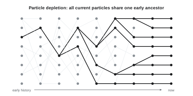
The fundamental limitation of particle-filter SLAM is particle depletion. The filter represents a distribution over whole trajectories, but resampling repeatedly throws away particles and duplicates others. After many resampling steps, all surviving particles descend from a few ancestors, so their histories, and therefore their maps, are nearly identical for the early part of the trajectory. When the robot finally closes a large loop, the filter needs a particle whose history happens to be consistent with the loop; if all particles share the same slightly wrong early history, none of them is, and the loop cannot be closed correctly. The longer the loop, the more particles are needed to keep enough diversity, and the number grows rapidly with loop length.
Remedies include better proposals (so fewer resamplings are needed), selective resampling, adaptive particle counts, and recovering diversity before a loop closure is expected. In practice, these methods work well for buildings with loops of a few hundred meters and struggle beyond that. Graph-based SLAM, which revisits the whole trajectory with an optimizer, has no equivalent limitation, which is the main reason it became dominant.
Worked problem
How depletion limits loop length
Suppose each resampling step keeps on average 60 % of distinct ancestors. A filter with 100 particles resamples every 2 m. Roughly how far can the robot travel before all particles share a single ancestor?
Show solution
- After n resamplings, distinct ancestors are about \( 100 \times 0.6^n \).
- Set \( 100 \times 0.6^n = 1 \): \( n = \ln(100)/\ln(1/0.6) = 4.605/0.511 = 9.0 \).
- Distance: \( 9 \times 2 = 18 \) m.
Answer: Under these assumptions, the trajectory history more than about 18 m back is shared by every particle. This simple model overstates the loss, but it shows why selective resampling and good proposals, which reduce the number of resamplings, are essential for closing loops.
| Method | Map per particle | Proposal | Typical particles | Strength |
|---|---|---|---|---|
| FastSLAM 1.0 | Landmark EKFs | Odometry | Hundreds to thousands | Per-particle data association |
| FastSLAM 2.0 | Landmark EKFs | Odometry plus measurement | Tens to hundreds | Works with few particles |
| GMapping | Occupancy grid | Scan-matching peak | 30–100 | Practical 2-D lidar SLAM |
Common mistakes
MistakeResampling at every step
InsteadResample only when the effective sample size falls below a threshold.
MistakeSampling new poses from odometry alone with an accurate lidar
InsteadUse an improved proposal that incorporates the measurement.
MistakeCopying every particle's full map on resampling
InsteadShare map structures between particles, for example in trees.
MistakeExpecting a fixed small particle count to close very large loops
InsteadRecognize particle depletion; use more particles, better proposals or a graph-based method.
MistakeForcing all particles to use the same data association
InsteadLet each particle choose its own association; this is a key robustness advantage.
Summary and key terms
- Given the trajectory, landmarks are conditionally independent, so the SLAM posterior factorizes.
- Rao-Blackwellized particle filters sample trajectories with particles and estimate each landmark or grid analytically per particle.
- FastSLAM gives each particle a pose and one small EKF per landmark, with per-particle data association.
- Particle weights are the measurement likelihoods under each particle's own map.
- FastSLAM 2.0 and GMapping use proposals that include the measurement, so few particles suffice.
- Selective resampling based on the effective sample size slows the loss of diversity.
- Particle depletion limits the size of loops that can be closed, favoring graph-based methods for large areas.
- Rao-Blackwellization
- Sampling some variables and computing the rest analytically given the samples.
- FastSLAM
- A Rao-Blackwellized particle filter with a small EKF per landmark in each particle.
- Importance weight
- A particle's weight, proportional to the likelihood of the measurements under it.
- Proposal distribution
- The distribution from which new particle poses are sampled.
- Improved proposal
- A proposal that incorporates the current measurement, not just odometry.
- GMapping
- A grid-based Rao-Blackwellized particle filter SLAM system for 2-D lidar.
- Effective sample size
- The quantity 1/Σw², measuring how many particles really contribute.
- Selective resampling
- Resampling only when the effective sample size is low.
- Particle depletion
- Loss of particle diversity through repeated resampling.
- Ancestor
- A particle from which current particles descend through resampling.
Practice problems
Work each problem on paper first, then reveal the answer to check.
Why are landmarks independent given the trajectory?
Show answer
They are connected only through the robot poses that observed them.
In FastSLAM, what does each particle store per landmark?
Show answer
A mean and a 2 × 2 covariance.
How does FastSLAM's memory scale with landmarks?
Show answer
Linearly, times the number of particles.
Innovation 0.1 m with variance 0.01 m²: unnormalized weight?
Show answer
\( \exp(-0.5) \approx 0.61 \).
Weights 0.25 each for four particles: N_eff?
Show answer
4.
Weights 0.9, 0.05, 0.05: N_eff?
Show answer
About 1.23.
What does GMapping's improved proposal use?
Show answer
A scan matcher to find the peak of the scan likelihood.
Why can each FastSLAM particle make its own data association?
Show answer
Each has its own map, so wrong choices die out in resampling.
What is particle depletion?
Show answer
Loss of diverse trajectory histories after repeated resampling.
Why does depletion matter for loop closure?
Show answer
No particle may have an early history consistent with the loop.
Lesson quiz · 5 questions
Score 60% or more to complete this lesson.
Create a free account to save your progress, take quizzes and earn a certificate.