
ROB-340 · Lesson 12 of 12 · 32 min
Capstone: a SLAM system for a warehouse robot
This capstone brings the course together in one design: a mapping and localization system for a fleet of autonomous mobile robots in a distribution warehouse. The scenario is fictional but typical. Northfield Logistics is commissioning 40 robots that tow carts between receiving, storage aisles and outbound docks in a 220 m by 140 m single-story building. The robots must localize to within 5 cm and 1° near pick-up and drop-off stations, run 20 hours a day, coexist with people and forklifts, and keep working as racking and stock change. The task is to choose sensors, a map representation, a SLAM and localization approach, a mapping procedure and a loop-closure strategy; to estimate whether the design meets its requirements; to plan its evaluation; and to analyze how it can fail. Planning and control (ROB-350) are out of scope except where they depend on localization.
Requirements
Good designs start from explicit, testable requirements. The table below lists those agreed with the operations team. Each one is measurable, so the evaluation plan can show whether it is met.
| ID | Requirement | Target | How verified |
|---|---|---|---|
| R1 | Position error at stations | ≤ 5 cm (95 %) | Total-station survey of docked poses |
| R2 | Heading error at stations | ≤ 1° (95 %) | Survey of two points on the robot |
| R3 | Position error in aisles | ≤ 15 cm (95 %) | Ground-truth runs with reflector targets |
| R4 | Localization availability | ≥ 99.9 % of operating time | Fleet logs of localization status |
| R5 | Recovery after power cycle or relocation | ≤ 30 s anywhere in the building | Kidnapping tests at 50 random poses |
| R6 | Map currency | Changes reflected within one shift | Scan-to-map agreement monitoring |
| R7 | Compute budget | ≤ 1 CPU core for localization | Profiling on the robot computer |
Sensors
Each robot already carries two safety-rated 2-D lidars at opposite corners, giving a 360° field of view at 25 cm height, as required for collision safety. Using the same scanners for localization avoids extra cost, though their 25 cm mounting height sees pallet loads and cart wheels as well as rack uprights and walls. The design adds a gyroscope-equipped IMU to the wheel odometry, and a forward-facing RGB-D camera that serves obstacle detection above scanner height and could later support visual features. A 3-D lidar was considered: it would see the ceiling and upper racking, which change less than floor-level stock, but at roughly ten times the cost per robot it was deferred as an option for problem areas.
Worked problem
Is the lidar accurate enough?
The safety lidars have a range noise of 2 cm (1σ) and an angular resolution of 0.25°. At a typical range of 6 m to rack uprights, what is the lateral spacing between beams, and does the noise allow 5 cm localization?
Show solution
- Beam spacing: \( 6 \times 0.25^{\circ} \times \pi/180 = 0.026 \) m.
- Each upright is hit by several beams per scan; a scan matcher averaging over hundreds of beams reduces the effect of 2 cm noise by roughly \( 1/\sqrt{n} \).
- With 300 informative beams, the noise contribution is about \( 0.02/\sqrt{300} \approx 1 \) mm.
Answer: Yes. Raw range noise is not the limiting factor; map quality, calibration, dynamic objects and geometry (degeneracy in aisles) dominate the error budget.
Map representation and approach
The 2-D lidars and the flat floor point to a 2-D occupancy grid at 5 cm for navigation, produced from a pose graph by graph-based SLAM (lesson 8). The pose graph itself is the master map, because it can be re-optimized, edited and extended, while the grid is a derived product. Commissioning uses slam_toolbox in mapping mode (lesson 9) with correlative scan matching and loop closure, and the robots then run slam_toolbox in localization mode against the serialized graph, with AMCL kept as a fallback, which gives precise scan-to-map matching with global relocalization. At the 1,750 stations, the robots switch to a dedicated docking mode that matches a local scan of the station's reflective markers, giving millimeter-level repeatability where it matters most.
Aisles are the hard part. Long rows of identical racking are both degenerate (little constraint along the aisle) and perceptually aliased (aisle 12 looks like aisle 13). The design addresses this three ways: wheel odometry and the gyroscope carry the estimate along aisles, where lidar constraint is weak; retroreflective tags at each aisle end, visible as high-intensity returns, break the aliasing; and the localizer reports degeneracy from the scan-matching Hessian (lesson 9) so the fusion filter down-weights lidar along the aisle.
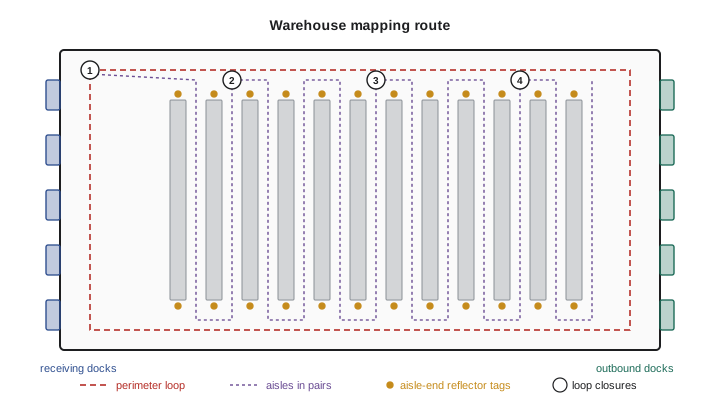
Mapping procedure and loop-closure strategy
The mapping run is planned rather than improvised. The site is mapped at night when it is quiet, with a robot driven at 0.5 m/s. The route first drives the full perimeter (about 720 m), returning to the start to close one large loop. It then covers the aisles in pairs, down one aisle and back up the next, crossing the main cross-aisle each time, so every pair creates a loop closure within a few hundred meters. Loop closures are accepted by slam_toolbox only above a conservative match score, and every accepted closure is reviewed afterwards in RViz, where the graph can be edited. After optimization, the grid is regenerated, people and parked equipment captured during mapping are erased, and keep-out zones and stations are annotated.
Worked problem
How often must loops be closed?
After calibration, the robot's fused odometry drifts at about 0.6 % of distance in aisles. The map in aisles must be accurate to about 10 cm (leaving room in the 15 cm requirement for localization noise). If error between closures is corrected linearly by the graph optimizer, so that the worst point is the middle of the stretch with about half the end error, how far apart can loop closures be?
Show solution
- End error before correction over distance D: \( 0.006 D \).
- After optimization, the worst error is roughly half of that: \( 0.003 D \).
- With odometry alone, require \( 0.003 D \le 0.10 \), so \( D \le 33 \) m. This is pessimistic, because the graph also uses scan matching to walls and racks along the way.
- With scan-matching constraints reducing effective drift to about 0.15 % in structured areas, \( D \le 0.10/0.00075 \approx 133 \) m.
Answer: Somewhere between about 35 m (odometry alone) and 130 m (with scan matching). Pairing aisles of about 120 m with a cross-aisle connection at each end keeps closures within this range.
import numpy as np
rng = np.random.default_rng(12)
def worst_error(route_len, spacing, gyro=0.0002, noise=0.01, trials=200):
    worst = []
    for _ in range(trials):
        s = np.arange(0, route_len, 1.0)
        heading = np.cumsum(rng.normal(0, gyro, len(s)))      # heading random walk (rad)
        err = np.cumsum(np.sin(heading)) + rng.normal(0, noise, len(s))   # lateral error (m)
        for start in np.arange(0, route_len, spacing):
            m = (s >= start) & (s < start + spacing)
            if m.sum() > 1:
                seg = err[m]; err[m] = seg - np.linspace(seg[0], seg[-1], m.sum())
        worst.append(np.percentile(np.abs(err), 95))
    return np.mean(worst)
for spacing in (50, 120, 300, 600):
print("loop closure every %4d m -> 95th-percentile map error %.3f m" % (spacing, worst_error(1200, spacing)))loop closure every 50 m -> 95th-percentile map error 0.029 m loop closure every 120 m -> 95th-percentile map error 0.062 m loop closure every 300 m -> 95th-percentile map error 0.212 m loop closure every 600 m -> 95th-percentile map error 0.522 m
With these illustrative parameters, closing loops about every 120 m keeps the 95th-percentile map error near 6 cm, inside the 10 cm target, while closures 300 m apart let it grow to about 20 cm. Because heading drift makes position error grow faster than linearly with distance, doubling the spacing more than doubles the error.
Error budget
The localization error at a station combines several independent sources, which add as a root sum of squares. The budget shows whether R1 is achievable and which term to improve first.
| Error source | Estimate (1σ) | Notes |
|---|---|---|
| Map error at station | 1.5 cm | Survey-checked after mapping |
| Scan-to-map matching | 1.0 cm | Station area well constrained |
| Lidar-to-robot extrinsic calibration | 0.8 cm | Includes 0.1° yaw at 4 m |
| Docking marker detection | 0.5 cm | Reflective markers at 1.5 m |
| Timing and motion during scan | 0.4 cm | Robot slows to 0.2 m/s |
Worked problem
Does the station budget meet R1?
Combine the error budget above by root sum of squares. Does the 95 % value meet the 5 cm requirement, assuming a 2-D Gaussian where the 95 % radius is about 2.45σ for each-axis σ?
Show solution
- \( \sigma = \sqrt{1.5^2 + 1.0^2 + 0.8^2 + 0.5^2 + 0.4^2} = \sqrt{2.25 + 1 + 0.64 + 0.25 + 0.16} = \sqrt{4.30} = 2.07 \) cm.
- 95 % radius: \( 2.45 \times 2.07 = 5.1 \) cm.
- This is just over 5 cm.
Answer: The design narrowly misses R1 on paper. The largest term is the map error, so the fix is to survey-correct the map at stations or rely on the docking markers alone near the station (removing the map term from the final approach): \( \sqrt{4.30 - 2.25} = 1.43 \) cm gives a 95 % radius of about 3.5 cm, which meets the requirement.
Evaluation plan
Verification follows the requirements table. Ground truth comes from a total station (a surveying instrument accurate to a few millimeters) that tracks a prism on the robot, plus surveyed reference points at a sample of stations. Test runs cover each zone (docks, aisles, cross-aisles) at normal speed and load, at different times of day to include people and forklift traffic. The team computes ATE after rigid alignment for map consistency, RPE over 10 m segments for drift, and station accuracy directly against surveyed poses (lesson 11). Kidnapping tests power-cycle robots at 50 random poses and measure time to relocalize (R5). A two-week shadow period runs the fleet with operators watching, logging localization status, recovery events and scan-to-map agreement per aisle (R4, R6). Acceptance requires every requirement to be met with margin on the measured data, not only in the budget.
Worked problem
Sizing the kidnapping test
R5 requires relocalization within 30 s. If the true failure rate were 5 %, what is the chance that 50 kidnapping trials would show no failures at all? What does that say about the test size?
Show solution
- Chance of no failures in 50 trials at 5 %: \( 0.95^{50} \).
- \( 0.95^{50} = e^{50 \ln 0.95} = e^{-2.565} = 0.077 \).
Answer: About 8 %, so a clean run of 50 trials gives roughly 92 % confidence that the failure rate is below 5 %. Demonstrating a rate below 1 % with similar confidence would need about 300 trials, which is why the shadow period logs real relocalizations as well.
Failure modes and mitigations
A failure mode and effects analysis lists how localization can fail, how each failure would be detected, and what the system does about it. The most important point is that every failure must be detectable: a robot that knows it is lost can stop safely and ask for help, while a robot that is confidently wrong is dangerous.
| Failure mode | Cause | Detection | Mitigation |
|---|---|---|---|
| Wrong aisle (aliasing) | Identical racking, weak prior | Reflector tag mismatch, multimodal belief | Aisle-end tags; slow down until resolved |
| Drift along aisle | Degenerate geometry | Small Hessian eigenvalue | Rely on odometry and gyro; tags at both ends |
| Map out of date | Moved racking or stock | Falling scan-to-map agreement by area | Lifelong mapping; scheduled local re-map |
| Kidnapping | Robot pushed or power-cycled | Likelihood drop, operator flag | Global relocalization; known start at charger |
| Sensor degradation | Dirty or misaligned lidar window | Intensity and return-rate monitoring | Maintenance alert; reduced speed |
| Dynamic clutter | People and forklifts in view | High fraction of unexplained beams | Filter detections; beam skipping |
| Software fault | Crash or timing overrun | Watchdog and heartbeat | Safe stop; restart and relocalize |
What this capstone shows
The design uses nearly every idea in the course. Calibrated odometry (lesson 1) carries the robot through degenerate aisles. The map is a pose graph that generates an occupancy grid (lessons 2, 4 and 8). Localization combines scan matching with particle-filter fallback and recovery (lesson 3). The mapping run is planned around the realities of SLAM, data association and loop closure (lesson 5), with lidar-specific front-end choices and degeneracy detection (lesson 9). Evaluation uses ATE, RPE and station surveys, and map maintenance relies on lifelong mapping (lesson 11). Filter-based SLAM (lessons 6 and 7) and visual SLAM (lesson 10) were considered and rejected for this site, with reasons recorded, which is itself part of good engineering. A design review would also ask what happens on a new site with different geometry, which is why the requirements, budgets and tests, not just the software configuration, are the real deliverables.
Common mistakes
MistakeStarting with a SLAM package instead of requirements
InsteadWrite measurable requirements first, then choose sensors and methods to meet them.
MistakeMapping with an improvised route
InsteadPlan the route to create loop closures within the drift budget.
MistakeAssuming raw sensor noise sets localization accuracy
InsteadBuild an error budget; map error, calibration and geometry usually dominate.
MistakeTesting only in quiet conditions
InsteadEvaluate with normal traffic, at different times, and over weeks of change.
MistakeAllowing failures that the robot cannot detect
InsteadDesign monitoring so the robot knows when it is lost and stops safely.
Summary and key terms
- A SLAM design starts from measurable requirements for accuracy, availability, recovery, currency and compute.
- Sensor choices balance cost, safety requirements and what the sensors see; raw noise is rarely the limit.
- A pose graph is the master map; occupancy grids and annotations are derived from it.
- Aisles are degenerate and aliased; odometry, aisle-end tags and degeneracy detection address them.
- The mapping route is planned so loop closures occur within the drift budget.
- Error budgets combine independent sources by root sum of squares and show which term to improve.
- Evaluation uses surveyed ground truth, ATE, RPE, kidnapping trials and a shadow period; every failure must be detectable.
- Requirement
- A measurable statement of what the system must achieve.
- Error budget
- An allocation of total allowed error among independent sources.
- Root sum of squares
- Combining independent errors as the square root of the sum of their squares.
- Total station
- A surveying instrument that measures positions to millimeters.
- Retroreflective tag
- A marker that returns lidar light strongly, giving a high-intensity return.
- Docking mode
- A precise local localization mode used near stations.
- Shadow period
- A supervised trial operation that logs performance before full release.
- FMEA
- Failure mode and effects analysis, a structured review of how a system can fail.
- Acceptance criteria
- Conditions that measured results must meet for the system to be accepted.
- Relocalization
- Recovering the pose in a known map after it has been lost.
Practice problems
Work each problem on paper first, then reveal the answer to check.
Why is the pose graph, not the grid, the master map?
Show answer
It can be re-optimized, edited and extended; the grid is derived from it.
Beam spacing at 8 m with 0.25° resolution?
Show answer
About 3.5 cm.
Drift 0.5 % and a 10 cm map target with linear correction (half-end error): maximum closure spacing?
Show answer
About 40 m.
Errors of 2, 1 and 2 cm combine by root sum of squares to?
Show answer
3 cm.
If σ per axis is 1.6 cm, about what is the 95 % radius?
Show answer
About 3.9 cm.
Chance of zero failures in 30 trials at a true 10 % failure rate?
Show answer
About 4 %.
Name a way to break aliasing between identical aisles.
Show answer
Retroreflective tags at aisle ends.
What signals that a map area is out of date?
Show answer
Falling scan-to-map agreement in that area.
Which metric checks global map consistency?
Show answer
ATE after alignment.
Why must every failure be detectable?
Show answer
A robot that knows it is lost can stop safely; a confidently wrong one is dangerous.
Lesson quiz · 5 questions
Score 60% or more to complete this lesson.
Create a free account to save your progress, take quizzes and earn a certificate.