
ROB-340 · Lesson 4 of 12 · 28 min
Occupancy grid mapping
Lesson 3 assumed the map was given. Where does it come from? The simplest version of the mapping problem assumes the opposite of localization: the robot's poses are known exactly, and the task is to build the map from the sensor readings. That assumption is never quite true, but it is a useful building block. It is exactly the situation inside many SLAM systems, which estimate the poses first and then build the grid from them, and it is how a map is rebuilt after a SLAM system has optimized its trajectory. This lesson derives the occupancy grid mapping algorithm, works through its log-odds update by hand, and discusses the practical choices that determine map quality: the inverse sensor model, resolution, thresholds and handling of dynamic objects.
The mapping problem with known poses
The full mapping problem is to estimate the posterior over maps given all measurements \( z_{1:t} \) and poses \( x_{1:t} \), written \( p(m \mid z_{1:t}, x_{1:t}) \). A map with a million cells, each occupied or free, has \( 2^{1{,}000{,}000} \) possible configurations, so this cannot be computed directly. Occupancy grid mapping makes a strong simplifying assumption: each cell is estimated independently of every other cell. The posterior factorizes into a product over cells,
and each cell becomes a binary estimation problem, occupied or free, with a static state. This independence assumption is wrong, because neighboring cells on a wall are strongly correlated, and it causes some artifacts discussed below, but it makes mapping fast and simple, and the results are good enough for most navigation.
The log-odds update
For a single binary static state, the Bayes filter becomes especially simple in log-odds form. The log-odds of a probability p is
Log-odds run from minus infinity (certainly free) through 0 (probability 0.5, unknown) to plus infinity (certainly occupied). In this form, the Bayes update for cell i after measurement \( z_t \) from pose \( x_t \) is a single addition:
Here \( p(m_i \mid z_t, x_t) \) is the inverse sensor model, the probability that the cell is occupied given only this one measurement, and \( \ell_0 \) is the prior log-odds, which is zero for a prior of 0.5. Addition avoids numerical trouble near 0 and 1, is cheap enough to run for every cell of every beam, and makes the result independent of the order of measurements. Implementations clamp the log-odds between limits (for example \( \pm 3.5 \), probabilities of about 0.03 and 0.97) so that cells can still change when the environment does.
Worked problem
Log-odds updates for one cell
An inverse sensor model assigns probability 0.7 to the cell where a beam ends (a hit) and 0.4 to cells the beam passes through (a miss). A cell starts unknown. It is hit three times and then missed once. What is its final occupancy probability?
Show solution
- Hit increment: \( \log(0.7/0.3) = 0.847 \). Miss increment: \( \log(0.4/0.6) = -0.405 \). Prior: \( \ell_0 = 0 \).
- After three hits: \( \ell = 3 \times 0.847 = 2.542 \).
- After one miss: \( \ell = 2.542 - 0.405 = 2.137 \).
- Probability: \( 1 - 1/(1 + e^{2.137}) = 1 - 1/9.47 = 0.894 \).
Answer: About 0.89, so the cell is confidently occupied. In log-odds, each hit and miss simply adds a fixed amount, which is why the update is so fast.
The inverse sensor model for a laser
For a range sensor, the inverse sensor model follows from the geometry of a beam. Cells along the beam between the sensor and the measured range are probably free, because the beam passed through them. The cell (or a thin band of cells) at the measured range is probably occupied, because something reflected the beam. Cells beyond the measured range are unknown, because the beam never reached them, and receive no update. Cells outside the beam's angular width are also untouched. A beam at the sensor's maximum range with no return is either discarded or used only to clear free space up to some distance, since a missing return gives no evidence of an obstacle.
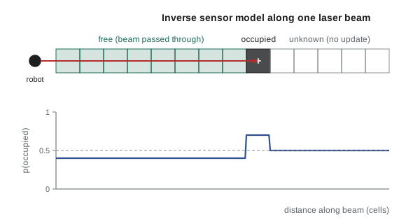
Finding the cells a beam passes through is a line-drawing problem. Bresenham's algorithm, invented in 1962 for pen plotters, steps along the line from the sensor cell to the endpoint cell using only integer additions, visiting each crossed cell once. For a 2-D lidar with 1,000 beams per scan at 10 Hz and beams up to 10 m long on a 5 cm grid, that is up to about 200 cells per beam and 2 million cell updates per second, well within a modern processor's reach. 3-D lidars produce far more beams, which is why 3-D mapping uses octrees, voxel hashing and GPU ray casting.
Worked problem
How many cells does one scan touch?
A 2-D lidar has 720 beams per scan. In a typical room the mean measured range is 4 m. On a 5 cm grid, roughly how many cell updates does one scan cause? At 15 scans per second?
Show solution
- Cells per beam: about \( 4/0.05 = 80 \) free cells plus one occupied.
- Per scan: \( 720 \times 81 \approx 58{,}000 \) updates.
- Per second at 15 Hz: about 870,000 updates.
Answer: Under a million simple additions a second, a small fraction of one CPU core. 2-D occupancy mapping is cheap; the expensive part of SLAM is getting the poses right.
import numpy as np
res, n = 0.1, 60                                  # 6 m x 6 m grid, 10 cm cells
L = np.zeros((n, n))                              # log-odds, 0 = unknown
l_hit, l_miss, lmax = np.log(0.7 / 0.3), np.log(0.4 / 0.6), 3.5
def bresenham(x0, y0, x1, y1):
    cells, dx, dy = [], abs(x1 - x0), -abs(y1 - y0)
    sx, sy, e = (1 if x0 < x1 else -1), (1 if y0 < y1 else -1), dx + dy
    while True:
        cells.append((x0, y0))
        if x0 == x1 and y0 == y1: return cells
        e2 = 2 * e
        if e2 >= dy: e += dy; x0 += sx
        if e2 <= dx: e += dx; y0 += sy
# square room walls at 1 m and 5 m; robot at (3, 3) takes 4 scans of 180 beams
def true_range(x, y, a):
    t = 0.0
    while 1.0 < x + t * np.cos(a) < 5.0 and 1.0 < y + t * np.sin(a) < 5.0: t += 0.01
    return t
rng = np.random.default_rng(0)
for _ in range(4):
    for a in np.linspace(-np.pi, np.pi, 180, endpoint=False):
        r = true_range(3.0, 3.0, a) + rng.normal(0, 0.02)
        ex, ey = 3.0 + r * np.cos(a), 3.0 + r * np.sin(a)
        ray = bresenham(30, 30, int(ex / res), int(ey / res))
        for (i, j) in ray[:-1]: L[j, i] = max(-lmax, L[j, i] + l_miss)
        i, j = ray[-1]; L[j, i] = min(lmax, L[j, i] + l_hit)
P = 1 - 1 / (1 + np.exp(L))
print("occupied cells (p > 0.65):", int((P > 0.65).sum()))
print("free cells (p < 0.35):    ", int((P < 0.35).sum()))
print("unknown cells:            ", int(((P >= 0.35) & (P <= 0.65)).sum()))
print("highest p near the wall x = 1 m on row y = 3 m: %.2f; p at the robot cell: %.2f" % (P[30, 8:12].max(), P[30, 30]))occupied cells (p > 0.65): 222 free cells (p < 0.35): 1448 unknown cells: 1930 highest p near the wall x = 1 m on row y = 3 m: 0.93; p at the robot cell: 0.03
Resolution, thresholds and map quality
Grid resolution trades detail against memory, computation and noise. A cell much smaller than the lidar's range noise or the pose uncertainty just spreads the same evidence over more cells, producing thick, fuzzy walls; a cell much larger than the robot's clearance hides doorways. For a 2-D lidar with a few centimeters of noise and good SLAM, 5 cm is the common default, with 2.5 cm for precise docking areas and 10 cm for large outdoor maps.
When a grid is saved for navigation, the probabilities are usually thresholded into three classes. ROS map_server's YAML file stores occupied_thresh (often 0.65) and free_thresh (often 0.196 or 0.25); cells above the first are obstacles, cells below the second are free, and those in between remain unknown. The navigation cost map then inflates obstacles by the robot's radius plus a safety margin.
Worked problem
Choosing a resolution
A robot with 0.6 m width must pass through 0.8 m doorways. Its lidar range noise is 3 cm and its localization accuracy is about 5 cm. Is a 10 cm grid acceptable? What about 5 cm?
Show solution
- Doorway margin: \( (0.8 - 0.6)/2 = 0.10 \) m on each side.
- With 10 cm cells, a wall edge can be misplaced by up to a cell, so a doorway can appear as narrow as 0.6 m, leaving no margin.
- With 5 cm cells, the quantization error is up to 5 cm, comparable to the localization error, leaving a usable margin.
Answer: Use 5 cm or finer. A 10 cm grid could make doorways look impassable. The cell size should be no larger than about half the smallest clearance the robot needs to resolve.
Artifacts and dynamic objects
The independence assumption and the simple inverse model produce characteristic artifacts. Walls seen at a glancing angle get thickened or partly erased, because beams that nearly graze a wall mark wall cells as free on the way past. Thin obstacles such as chair legs may be hit by some beams and passed by others, so they flicker between occupied and free. Glass and mirrors produce no return or a return from the wrong place. Black or very shiny surfaces return weakly. More sophisticated inverse models account for beam width and incidence angle, and forward-model mapping methods estimate the most likely map jointly rather than cell by cell, at higher cost.
Dynamic objects leave trails. A person walking past the robot is marked occupied wherever they were seen, until later beams pass through those cells and clear them. Clamping log-odds keeps cells changeable, and using a slightly larger miss increment than hit increment lets the map forget transient objects faster. Some systems detect and remove moving objects before mapping, or build the map only from scans taken when the area is empty. Long-term map maintenance, where the robot updates a deployed map as the environment changes, is covered in lesson 11.
| Choice | Typical value | Why |
|---|---|---|
| Resolution (2-D lidar, indoors) | 5 cm | Matches lidar noise and localization accuracy |
| Hit probability | 0.6–0.75 | Strength of evidence from a return |
| Miss probability | 0.35–0.45 | Strength of evidence from a pass-through |
| Log-odds clamp | About ±3.5 | Keeps cells able to change |
| occupied_thresh / free_thresh | 0.65 / 0.25 | Three-class map for navigation |
| Maximum range used | Below the sensor maximum | Avoid noisy long beams and max-range readings |
From mapping to SLAM
Occupancy grid mapping with known poses is easy; the difficulty is that the poses are not known. If odometry is used as the poses, the map warps as odometry drifts: corridors bend, rooms overlap, and a loop around a building fails to close. The rest of this course is about estimating the poses well enough that the map comes out right. Some SLAM methods (Rao-Blackwellized particle filters, lesson 7) carry a grid per particle; others (graph SLAM, lesson 8) optimize the trajectory and then build the grid once from the corrected poses. Either way, the grid-building step is the one from this lesson.
Common mistakes
MistakeUpdating probabilities directly by multiplication near 0 and 1
InsteadUse log-odds, where the update is a stable addition.
MistakeLetting log-odds grow without limit
InsteadClamp them so that cells can change when the environment does.
MistakeMarking cells beyond the measured range as free
InsteadLeave cells beyond the return unknown; the beam never reached them.
MistakeTreating max-range readings as hits
InsteadDiscard them or use them only to clear free space up to a limit.
MistakeBuilding a map from raw odometry poses over a long run
InsteadCorrect the poses with SLAM first; drift warps the map.
Summary and key terms
- Occupancy grid mapping estimates each cell's occupancy independently, given known poses.
- In log-odds form, the Bayes update for a cell is a single addition of the inverse sensor model term.
- The laser inverse sensor model marks cells before the return as free, the return cell as occupied and cells beyond as unknown.
- Bresenham's algorithm finds the cells along each beam using integer steps.
- Resolution should be no larger than about half the smallest clearance the robot must resolve.
- Thresholds turn probabilities into occupied, free and unknown classes for navigation.
- Wrong poses warp the map, which is why mapping needs SLAM.
- Log-odds
- The logarithm of p/(1 − p), which turns Bayes updates into additions.
- Inverse sensor model
- The probability that a cell is occupied given a single measurement.
- Prior log-odds
- The log-odds before any measurement, zero for p = 0.5.
- Bresenham's algorithm
- An integer method for listing the grid cells along a line.
- Clamping
- Limiting log-odds to a range so cells stay changeable.
- occupied_thresh
- The probability above which a saved map cell is treated as an obstacle.
- free_thresh
- The probability below which a saved map cell is treated as free.
- Max-range reading
- A beam that returned no echo within the sensor's range.
- Static world assumption
- The assumption that the mapped environment does not change.
- Ray casting
- Tracing a beam through a map to find the cells it crosses or the first obstacle.
Practice problems
Work each problem on paper first, then reveal the answer to check.
What log-odds corresponds to probability 0.5?
Show answer
0.
Convert log-odds 1.0 to a probability.
Show answer
About 0.73.
Hit probability 0.8: what is the log-odds increment?
Show answer
\( \log 4 \approx 1.386 \).
A cell receives two hits of +0.85 and two misses of −0.41. What is its log-odds?
Show answer
0.88, probability about 0.71.
Which cells along a beam receive no update?
Show answer
Cells beyond the measured range.
Why are log-odds clamped?
Show answer
So that cells can change if the environment changes.
A robot must resolve 0.12 m clearances. What maximum resolution is sensible?
Show answer
About 6 cm or finer.
Name two common grid artifacts.
Show answer
Thickened or eroded walls at glancing angles, flickering thin obstacles, trails of moving people, glass gaps.
What does a cell between free_thresh and occupied_thresh become in a saved map?
Show answer
Unknown.
Why does a map built from raw odometry warp?
Show answer
Odometry drift puts later scans in the wrong place.
Lesson quiz · 5 questions
Score 60% or more to complete this lesson.
Create a free account to save your progress, take quizzes and earn a certificate.