Measuring before optimizing

Ridgeline Coffee Roasters has grown into its software. The tools Jordan Reyes wrote in PYTH-101 and turned into the ridgeline package in PYTH-102 now run every day, and some of them have become slow. Anita Shah's month-end sales report, which took two seconds when the shop sold six coffees to a handful of regulars, now takes several minutes on three years of sales. Kai Nakamura's roaster records a temperature every second, so a busy week produces hundreds of thousands of readings, and the script that draws his roast curves makes him wait. Theo Barnes asks for shipping quotes one order at a time, and on a Monday with two hundred weekend orders that loop runs for well over a minute.

Jordan's first instinct is to start rewriting things to make them faster. This course begins by resisting that instinct. Speeding up a program is an engineering task with a method: decide what fast enough means, measure where the time actually goes, change the one thing that matters most, and measure again. This lesson covers that method: performance goals, timing code properly with time.perf_counter and timeit, counting the work a program does, the big-O vocabulary for how work grows with input size, and Amdahl's law, which tells you how much any single improvement can possibly help.

Fast enough is a requirement, not a feeling

Before changing any code, write down what you are trying to achieve, in numbers. Performance has several dimensions, and improving one can hurt another. Latency is how long one request or task takes: how long Theo waits for one shipping quote, or how long a product page takes to show. Throughput is how much work is done per unit of time: how many orders an hour the shop can process, or how many roast readings a second the analysis can handle. Resource use is how much memory, processor time, disk or network a task consumes. A change that makes one report faster by loading everything into memory can also make it use four times the memory.

A useful performance goal names the task, the size of the input and the limit. Ridgeline's goals, agreed with Rosa Delgado at a Monday meeting, look like this:

• The month-end report must finish in under 10 seconds on three years of sales, about 150,000 sale lines.
• The product page stock check must answer in under 50 milliseconds.
• Monday shipping quotes for 200 orders must finish in under 15 seconds.
• Kai's roast-curve analysis for one week of readings must finish in under 5 seconds.

Look at what these goals leave out. They do not ask for the code to be as fast as possible, which would never end. They say when the work is done. A report that takes 8 seconds meets its goal, and spending a week to get it to 2 seconds is a poor use of Jordan's time when the Monday quotes still take over a minute. Goals also tell you when to stop: once each task meets its limit, the remaining time is better spent on features and correctness.

Why guessing fails

Programmers are notoriously bad at guessing where their programs spend time. The slow part is often not the code that looks complicated but an innocent line inside a loop that runs a million times, or a call to a library function that hides a slow operation. Donald Knuth's often-quoted warning is that premature optimization is the root of much evil in programming: effort spent speeding up code that does not matter makes the program harder to read and maintain, and gains nothing.

Jordan learned this the hard way. Convinced that the month-end report was slow because of the f-string formatting in the final table, he spent an afternoon replacing it with string concatenation. The report took exactly as long as before, because the formatting ran once per coffee, six times in total, while the real problem was elsewhere. The rule for this course is simple: no optimization without a measurement that shows the problem, and no optimization is finished until a second measurement shows the improvement.

Timing code with time.perf_counter

The simplest measurement is wall-clock time: note the time before a piece of code runs, note it after, and subtract. Python's time.perf_counter() returns a high-resolution clock value in seconds, meant exactly for this. Its value on its own means nothing; only the difference between two readings matters. Unlike time.time(), it is not affected by changes to the system clock.

import time

def slow_total(n):
    total = 0
    for i in range(n):
        total += i * i
    return total

start = time.perf_counter()
result = slow_total(200_000)
elapsed = time.perf_counter() - start
print("result:", result)
print(f"took {elapsed:.4f} seconds")

result: 2666646666700000
took 0.0097 seconds

Run this a few times and the printed time changes, even though the code does exactly the same work. Timing measurements are noisy. Other programs share the processor, the operating system interrupts your program, caches warm up after the first run, and in a browser the page itself competes for time. One measurement is a rough indication, not a fact. Professional measurement repeats the work many times and looks at the best or the typical result.

There is also a scale problem. A function that takes a few microseconds cannot be timed reliably with one call, because the clock resolution and the overhead of calling perf_counter itself are of the same size. The fix is to run the code many times in a loop and divide.

The timeit module

The standard library's timeit module does careful repeated timing for you. timeit.timeit() runs a statement a given number of times and returns the total time; timeit.repeat() does that several times so you can see the spread. It also switches off the garbage collector during the measurement by default, which removes one source of noise. The usual practice is to take the minimum of the repeated results, because noise only ever adds time: the fastest run is the closest to the true cost of the code.

import timeit

codes = [f"RC-{n}" for n in range(1000)]
as_set = set(codes)

list_times = timeit.repeat(lambda: "RC-999" in codes, number=2000, repeat=5)
set_times = timeit.repeat(lambda: "RC-999" in as_set, number=2000, repeat=5)
best_list = min(list_times) / 2000
best_set = min(set_times) / 2000
print(f"list membership: {best_list * 1e6:.2f} microseconds")
print(f"set membership:  {best_set * 1e6:.3f} microseconds")
print("set is faster:", best_set < best_list)

list membership: 6.27 microseconds
set membership:  0.030 microseconds
set is faster: True

From the command line, python -m timeit runs a quick experiment without writing a script, and in Jupyter notebooks the %timeit magic does the same. Whichever form you use, the comparison is what matters: a list membership test for the last of a thousand codes checks every element, while a set finds it almost instantly. The exact numbers depend on the machine, but the ratio between them is stable and meaningful.

> python -m timeit -s "codes = [f'RC-{n}' for n in range(1000)]" "'RC-999' in codes"
20000 loops, best of 5: 11.2 usec per loop
> python -m timeit -s "codes = {f'RC-{n}' for n in range(1000)}" "'RC-999' in codes"
10000000 loops, best of 5: 22.6 nsec per loop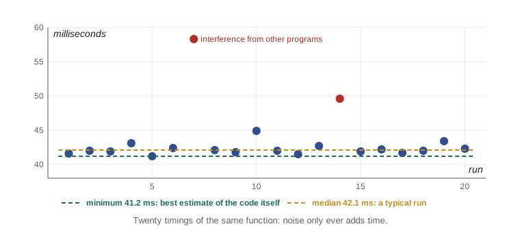

Counting work instead of seconds

Seconds depend on the machine, the load and the phase of the moon. The amount of work an algorithm does does not. Counting operations, such as comparisons, loop iterations or dictionary lookups, gives a measurement that is the same on every run and every computer. It is also how you compare approaches before running them on real data. Here Jordan counts how many comparisons it takes to find a sale's coffee by searching a list, against looking it up in a dictionary.

coffees = [(f"RC-{n}", f"Coffee {n}") for n in range(101, 101 + 600)]

def find_in_list(code, items):
    comparisons = 0
    for c, name in items:
        comparisons += 1
        if c == code:
            return name, comparisons
    return None, comparisons

index = dict(coffees)                    # built once: code -> name

for code in ["RC-101", "RC-400", "RC-700"]:
    name, steps = find_in_list(code, coffees)
    print(f"{code}: list search took {steps} comparisons, dict lookup 1 hash step -> {index[code]}")

sales = 150_000
avg = sum(find_in_list(c, coffees)[1] for c, _ in coffees) / len(coffees)
print(f"average list search: {avg:.1f} comparisons")
print(f"for {sales:,} sale lines: about {sales * avg:,.0f} comparisons vs {sales:,} lookups")

RC-101: list search took 1 comparisons, dict lookup 1 hash step -> Coffee 101
RC-400: list search took 300 comparisons, dict lookup 1 hash step -> Coffee 400
RC-700: list search took 600 comparisons, dict lookup 1 hash step -> Coffee 700
average list search: 300.5 comparisons
for 150,000 sale lines: about 45,075,000 comparisons vs 150,000 lookups

The count makes the problem plain. Matching each of 150,000 sale lines to its coffee by searching a list of 600 products costs about 45 million comparisons, while a dictionary does 150,000 lookups. No timing noise can hide a factor of three hundred. This is the kind of evidence that should drive an optimization.

Big-O: how work grows

Counting work for one input size is useful; knowing how the count grows as the input grows is better. Big-O notation describes that growth, ignoring constant factors and small terms. A list search is O(n): double the list and the work doubles. A dictionary or set lookup is O(1) on average: the work stays the same no matter how many items there are. Sorting with Python's built-in sort is O(n log n). Checking every pair of items, as a naive duplicate finder does, is O(n²): double the input and the work quadruples.

import math

print(f"{'n':>9} {'log n':>7} {'n':>9} {'n log n':>11} {'n squared':>16}")
for n in [10, 1_000, 100_000, 1_000_000]:
    print(f"{n:>9,} {math.log2(n):>7.1f} {n:>9,} {n * math.log2(n):>11,.0f} {n * n:>16,}")

        n   log n         n     n log n        n squared
       10     3.3        10          33              100
    1,000    10.0     1,000       9,966        1,000,000
  100,000    16.6   100,000   1,660,964   10,000,000,000
1,000,000    19.9 1,000,000  19,931,569 1,000,000,000,000

The table shows why algorithm choice dominates everything else at scale. At ten items every approach is instant. At a million items, an O(n log n) sort does about twenty million steps, while an O(n²) pairwise check does a trillion, which at a hundred million simple steps a second is close to three hours. Rewriting an O(n²) algorithm as O(n log n) or O(n) is worth more than any amount of fine-tuning of the inner loop.

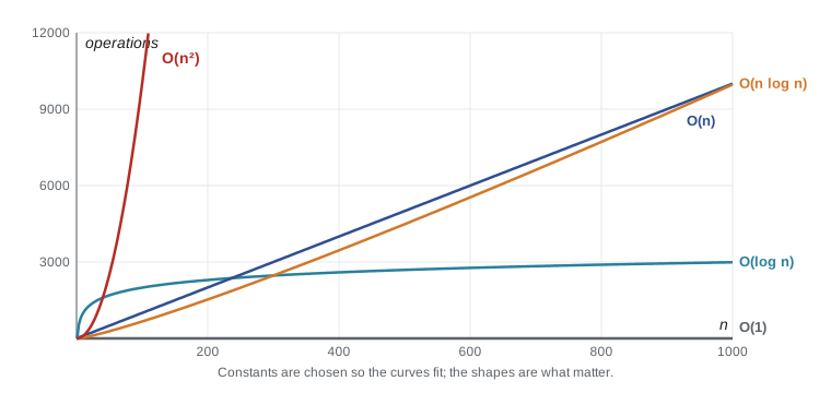
Big-O hides constants, and constants matter at small sizes. A clever O(n log n) algorithm can be slower than a simple O(n²) one for ten items. Python's built-in functions, written in C, also have small constants, which is why sum(), sorted() and set operations usually beat equivalent hand-written loops. Big-O tells you how a program will behave as the data grows; measurement tells you how it behaves today.

Amdahl's law: the limit of any single fix

Suppose Jordan's profiling shows that the month-end report spends 80 parts in 100 of its time matching sales to coffees and the rest reading the file and printing. Even if he made the matching infinitely fast, the report could only become five times faster, because the reading and printing would still take their 20 parts. This is Amdahl's law: the overall speedup from improving one part of a program is limited by the fraction of time that part takes.

If a fraction p of the running time is sped up by a factor s, the new time is (1 - p) + p / s of the old time, and the overall speedup is 1 / ((1 - p) + p / s). The law applies to every kind of optimization, and it is especially important for parallel computing, where s is the number of processors: a program that is 10 parts in 100 sequential can never run more than ten times faster, no matter how many cores it uses.

def amdahl(p, s):
    """Overall speedup when a fraction p of the time is made s times faster."""
    return 1 / ((1 - p) + p / s)

for p in [0.5, 0.8, 0.95]:
    row = [f"{amdahl(p, s):5.2f}" for s in (2, 4, 10, 1000)]
    print(f"p = {p:.2f}: speedups for s = 2, 4, 10, 1000 ->", "  ".join(row))

print("matching 80 of 100 parts, made 50x faster:", round(amdahl(0.8, 50), 2))

p = 0.50: speedups for s = 2, 4, 10, 1000 ->  1.33   1.60   1.82   2.00
p = 0.80: speedups for s = 2, 4, 10, 1000 ->  1.67   2.50   3.57   4.98
p = 0.95: speedups for s = 2, 4, 10, 1000 ->  1.90   3.48   6.90  19.63
matching 80 of 100 parts, made 50x faster: 4.63

The numbers show the practical lesson. Speeding up a part that takes half the time by a factor of a thousand gives barely a factor of two overall. Speeding up the part that takes 95 parts in 100 by a factor of ten gives almost seven. Always work on the biggest slice of time first, and expect diminishing returns as each slice shrinks and the others become the bottleneck.

def amdahl(p, s):
    return p * s

def max_speedup(p):
    return 0

print(round(amdahl(0.8, 50), 2))

Measure the right thing

A measurement is only useful if it reflects real use. Timing the month-end report on a test file of ten sales tells Jordan nothing about three years of sales, because the slow part grows with the data. Good benchmarks use realistic input sizes, include the slow cases as well as the typical ones, and time the whole task a user waits for, not just the function that is easy to time. They also check that the result is still correct: a faster program that gives the wrong total is not an optimization.

It also pays to keep the measurement. A small benchmark script, saved in the repository next to the tests, lets anyone rerun the measurement after a change and catch a performance regression, a change that accidentally makes things slower. Jordan adds bench_report.py to the ridgeline repository: it generates a realistic year of fake sales with a fixed random seed, times the report three times and prints the best time and the total, so the result can be compared before and after every change.

import random

def fake_sales(n, seed=2026):
    """Realistic but reproducible sale lines: (sku, qty)."""
    rnd = random.Random(seed)
    skus = [f"RC-{c}" for c in range(101, 107)]
    weights = [30, 10, 18, 6, 8, 28]          # best sellers sell more
    return [(rnd.choices(skus, weights)[0], rnd.randint(1, 3)) for _ in range(n)]

sales = fake_sales(10_000)
print(len(sales), "sales, first three:", sales[:3])
print("same data every time:", fake_sales(5) == fake_sales(5))
totals = {}
for sku, qty in sales:
    totals[sku] = totals.get(sku, 0) + qty
print(dict(sorted(totals.items())))

10000 sales, first three: [('RC-101', 3), ('RC-106', 3), ('RC-106', 1)]
same data every time: True
{'RC-101': 6105, 'RC-102': 2016, 'RC-103': 3453, 'RC-104': 1261, 'RC-105': 1521, 'RC-106': 5531}

def linear_steps(items, target):
    return 1

def binary_steps(items, target):
    return 1

data = list(range(0, 2000, 2))
print(linear_steps(data, 1998), binary_steps(data, 1998))

A method for every optimization

The rest of this course follows the same loop for every change, and it is worth stating plainly. First, set a goal in numbers. Second, measure the current behavior with a realistic benchmark. Third, profile to find where the time goes, the subject of the next lesson. Fourth, change the single biggest cost, preferring a better algorithm or data structure over clever tricks. Fifth, check the results are still correct and measure again. Stop when the goal is met.

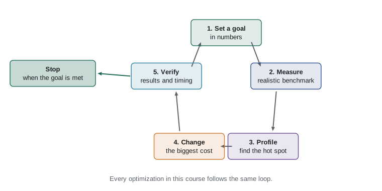
The techniques in later lessons, threads, processes, asyncio, NumPy and caching, are all tools for step four. Each suits a particular kind of slowness. Code that waits for networks and disks needs concurrency; code that crunches numbers needs better algorithms, vectorized libraries or more processors; code that repeats the same work needs caching. Knowing which kind of slowness you have is the job of measurement.