Atmospheric dynamics: Coriolis, geostrophic wind and circulation

Air flows from high pressure to low pressure, yet a weather map shows something stranger: away from the ground, the wind blows almost exactly along the isobars, the lines of constant pressure, circling clockwise around high-pressure systems and counterclockwise around lows in the northern hemisphere. It does not flow straight into the low and fill it. The reason is the rotation of the Earth. On a rotating planet, large-scale air motion is governed by a balance between the pressure-gradient force and the Coriolis force, met for a single particle in PHYS-244. This lesson writes the equations of motion in the rotating frame, derives the geostrophic and thermal wind balances, uses the Rossby number to decide when rotation matters, and then explains the general circulation of the atmosphere: the trade winds, the westerlies, the jet streams and the three-cell picture of Hadley, Ferrel and polar cells.

The equations of motion in a rotating frame

PHYS-244 showed that in a frame rotating with angular velocity \(\boldsymbol{\Omega}\), Newton's second law acquires two fictitious forces per unit mass: the centrifugal force \(-\boldsymbol{\Omega}\times(\boldsymbol{\Omega}\times\mathbf{r})\) and the Coriolis force \(-2\boldsymbol{\Omega}\times\mathbf{v}\). For the atmosphere, the centrifugal force is absorbed into effective gravity, which is why \(g\) varies slightly with latitude and why the Earth is slightly flattened. Including the pressure-gradient force \(-\nabla p/\rho\) and friction \(\mathbf{F}\), the momentum equation for air is

where \(D/Dt\) is the derivative following the moving air. The Earth's rotation rate is \(\Omega = 2\pi/(23.93\ \text{h}) = 7.292\times10^{-5}\) s\(^{-1}\), using the sidereal day. For horizontal motion, only the vertical component of \(\boldsymbol{\Omega}\), \(\Omega\sin\phi\) at latitude \(\phi\), matters for the horizontal Coriolis force. Defining the Coriolis parameter

the horizontal Coriolis force per unit mass is \(-f\,\hat{\mathbf{z}}\times\mathbf{v}\): it acts at right angles to the velocity, to the right of the motion in the northern hemisphere and to the left in the southern. It is zero at the equator, where the vertical component of the rotation vanishes, and largest at the poles.

Scale analysis and the Rossby number

Whether rotation matters depends on how long the motion lasts compared with a day. Compare the acceleration term, of order \(U^2/L\) for a speed \(U\) and length scale \(L\), with the Coriolis term \(fU\). Their ratio is the Rossby number

When \(\mathrm{Ro} \ll 1\), rotation dominates and the flow is close to geostrophic balance. When \(\mathrm{Ro} \gg 1\), rotation is negligible and the flow is governed by pressure gradients, inertia and friction alone. The program below evaluates \(f\) at Minneapolis and elsewhere, computes geostrophic winds, the thermal wind shear and the gradient wind, and tabulates the Rossby number for flows from a bathtub drain to a mid-latitude cyclone.

import math
Omega = 7.2921e-5
cities = [("Winnipeg", 49.9), ("Minneapolis", 44.98)]
print("Coriolis parameter f = 2 Omega sin(latitude)")
for name, phi in [("equator", 0.0)] + cities + [("North Pole", 90.0)]:
    f = 2 * Omega * math.sin(math.radians(phi))
    print(f"  {name:12s} f = {f:.3e} 1/s", "" if f == 0 else f"inertial period {2 * math.pi / f / 3600:.1f} h")

rho = 1.2; dp = 400.0; dx = 300e3   # 4 hPa change over 300 km
for name, phi in cities:
    fc = 2 * Omega * math.sin(math.radians(phi))
    print(f"geostrophic wind for 4 hPa per 300 km at {name}: {dp / dx / (rho * fc):.1f} m/s = {dp / dx / (rho * fc) * 3.6:.0f} km/h")
f = 2 * Omega * math.sin(math.radians(45.0))   # use 45 degrees for the rest
vg = dp / dx / (rho * f)
print(f"at 45 degrees: f = {f:.3e} 1/s, geostrophic wind {vg:.1f} m/s")
# at 500 hPa height gradients: 60 m over 500 km
g = 9.81
vg500 = g / f * 60 / 500e3
print(f"500 hPa: 60 m height change over 500 km -> {vg500:.1f} m/s")

# Thermal wind: shear from a horizontal temperature gradient
dTdy = -10 / 1000e3   # 10 K colder per 1000 km northward
T = 260.0
shear = -g / (f * T) * dTdy
print(f"thermal wind shear = {shear * 1000:.2f} m/s per km -> {shear * 10000:.0f} m/s over 10 km of height")

# Rossby numbers
for name, U, Lscale in [("bathtub vortex", 0.1, 0.1), ("tornado", 50, 300), ("thunderstorm", 10, 10e3),
                       ("hurricane", 40, 300e3), ("mid-latitude cyclone", 10, 1000e3)]:
    Ro = U / (f * Lscale)
    print(f"Rossby number, {name:22s} {Ro:9.3g}")

# Gradient wind: curvature correction for a low of radius 500 km
R = 500e3
vgr = (-f * R / 2) + math.sqrt((f * R / 2) ** 2 + f * R * vg)
print(f"gradient wind around a low (R = 500 km): {vgr:.1f} m/s, slower than geostrophic {vg:.1f} m/s")

Coriolis parameter f = 2 Omega sin(latitude)
  equator      f = 0.000e+00 1/s 
  Winnipeg     f = 1.116e-04 1/s inertial period 15.6 h
  Minneapolis  f = 1.031e-04 1/s inertial period 16.9 h
  North Pole   f = 1.458e-04 1/s inertial period 12.0 h
geostrophic wind for 4 hPa per 300 km at Winnipeg: 10.0 m/s = 36 km/h
geostrophic wind for 4 hPa per 300 km at Minneapolis: 10.8 m/s = 39 km/h
at 45 degrees: f = 1.031e-04 1/s, geostrophic wind 10.8 m/s
500 hPa: 60 m height change over 500 km -> 11.4 m/s
thermal wind shear = 3.66 m/s per km -> 37 m/s over 10 km of height
Rossby number, bathtub vortex           9.7e+03
Rossby number, tornado                 1.62e+03
Rossby number, thunderstorm                 9.7
Rossby number, hurricane                   1.29
Rossby number, mid-latitude cyclone       0.097
gradient wind around a low (R = 500 km): 9.2 m/s, slower than geostrophic 10.8 m/s

The Rossby number of a bathtub vortex is about 10 000 and that of a tornado about 1600, so the Earth's rotation has nothing to do with the direction either one spins: both depend on the initial motion of the water or air. The popular claim that bathtubs drain one way north of the equator and the other way south is false; careful experiments that remove all other motion can detect the Coriolis effect, but ordinary drains cannot. A thunderstorm, with \(\mathrm{Ro} \approx 10\), feels rotation only weakly. A hurricane, with \(\mathrm{Ro}\) near 1, feels it strongly, which is why hurricanes spin counterclockwise in the north. A mid-latitude cyclone, with \(\mathrm{Ro} \approx 0.1\), is dominated by rotation.

Geostrophic balance

When \(\mathrm{Ro} \ll 1\) and friction is small, as it is above the lowest kilometer, the horizontal momentum equation reduces to a balance between the pressure-gradient force and the Coriolis force:

The geostrophic wind \(\mathbf{v}_g\) blows parallel to the isobars, with low pressure on its left in the northern hemisphere: this is Buys Ballot's law of 1857. Its speed is proportional to the pressure gradient, so closely spaced isobars mean strong winds. In the program, a gradient of 4 hPa over 300 km gives a geostrophic wind of about 10.8 m/s at Minneapolis, a typical value. Meteorologists usually work on pressure surfaces rather than at constant height, and then the geostrophic wind is \(\mathbf{v}_g = (g/f)\,\hat{\mathbf{z}}\times\nabla_p Z\), where \(Z\) is the height of the pressure surface; a height change of 60 m over 500 km on a 500 hPa chart gives about 11 m/s at 45°.

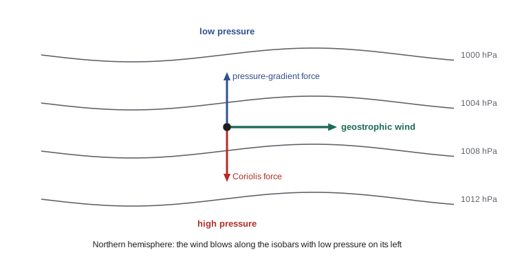
Geostrophic balance is a diagnostic relation, not a prediction: it tells you the wind that goes with a given pressure field but not how the field evolves. The small departures from balance, the ageostrophic wind, are what make weather systems develop, and computing them is the heart of numerical weather prediction. Near the ground, friction slows the wind, the Coriolis force weakens with it, and the pressure-gradient force wins slightly: the wind turns across the isobars toward low pressure by 10 to 30 degrees over the ocean and more over rough land. This frictional inflow converges into low-pressure centers, forcing air upward, which is why lows bring clouds and precipitation while highs bring sinking air and clear skies.

Gradient wind and curved flow

Around a low with curved isobars, the air must also accelerate toward the center of curvature, which requires a net inward force. The gradient wind balance adds the centripetal term: \(V^2/R + fV = (1/\rho)\,\partial p/\partial n\) around a low of radius \(R\). Solving the quadratic shows that the wind around a low is slower than the geostrophic value, while around a high it is faster; in the program, the geostrophic 10.8 m/s at 45° becomes 9.2 m/s around a low of radius 500 km. The asymmetry also limits highs: around a high, the gradient wind equation has real solutions only if the pressure gradient is weak, which is why anticyclones have gentle pressure gradients and light winds in their centers, while lows can have steep gradients and strong winds.

The thermal wind

Geostrophic balance combined with hydrostatic balance links horizontal temperature gradients to vertical wind shear. Because cold air columns are shallower than warm ones, pressure surfaces slope down toward cold air, and the slope increases with height. The result, the thermal wind equation, is

In the northern hemisphere, with colder air to the north, the westerly wind increases with height. A temperature difference of 10 K per 1000 km at 45° gives a shear of about 3.7 m/s per km, about 37 m/s across the troposphere, so a westerly of a few meters per second at the ground becomes a jet of 40 m/s near the tropopause. The polar jet stream is concentrated above the polar front, where the temperature gradient between polar and mid-latitude air is sharpest, and it is strongest in winter, when that gradient is largest. Its meanders, the long Rossby waves several thousand kilometers across, steer storms across the continent and bring cold Arctic outbreaks south when they dip deeply.

The general circulation

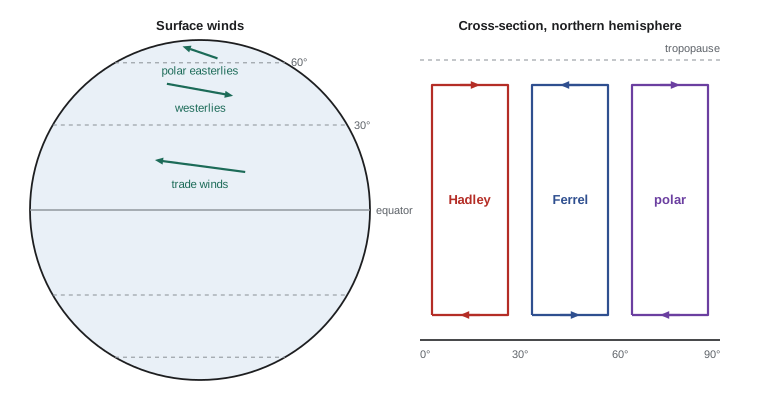
The tropics absorb more sunlight than they radiate, and the polar regions radiate more than they absorb, so the atmosphere and oceans must carry about 5 PW of heat poleward in each hemisphere. In 1735 George Hadley proposed a single overturning cell in each hemisphere: warm air rising at the equator, flowing poleward aloft, sinking at the poles and returning along the surface, with the Earth's rotation turning the returning air into easterly trade winds. The rising branch near the equator exists; it forms the intertropical convergence zone, a band of deep thunderstorms. But angular momentum conservation prevents the cell from reaching the pole. Air moving poleward aloft from the equator, conserving its angular momentum about the Earth's axis, would reach a westerly speed of about 130 m/s at 30 degrees latitude. Such strong winds are unstable, and the Hadley cell ends near 30 degrees, where the air sinks, warms adiabatically and forms the belt of subtropical highs and deserts.

Poleward of 30 degrees, the heat is carried not by a steady overturning cell but by the large eddies, the cyclones and anticyclones of mid-latitude weather, that develop from the instability of the westerly jet; this process is called baroclinic instability. Averaged around latitude circles, the eddies produce a weak reverse circulation, the Ferrel cell that William Ferrel described in 1856, with surface westerlies between about 30 and 60 degrees. A weaker polar cell, with sinking air over the pole and surface polar easterlies, completes the picture. The three-cell model is a zonal average and should not be taken literally on a given day, but it explains the global pattern of surface winds, deserts, rain belts and storm tracks.

The Canadian Prairies and the northern United States lie under the westerlies and near the mean position of the polar front, so their weather is dominated by the passage of mid-latitude cyclones, typically every three to five days, alternating with outbreaks of cold Arctic air in winter. Lows that form in the lee of the Rockies in Alberta, called Alberta clippers, race southeastward across the Prairies and the Great Lakes, while lows that form in the lee of the Colorado Rockies bring heavy snow to the northern plains.