The magnetosphere: dipole field, magnetopause and radiation belts

The Earth's magnetic field is weak at the surface, about 30 to 60 µT, a hundredth of a fridge magnet's, yet it shields the planet from the solar wind out to about ten Earth radii and traps a population of energetic particles that would be lethal to an unprotected astronaut. The region it controls is the magnetosphere. This lesson models the field as a dipole, finds where the solar wind's pressure balances the field's pressure at the magnetopause, describes the overall shape of the magnetosphere with its bow shock and long tail, and then follows individual charged particles: their gyration around field lines, their bounce between magnetic mirrors, and their slow drift around the Earth. A numerical particle pusher integrates the motion of a 10 MeV proton in the radiation belts and checks all three motions against theory.

The dipole field

To a good first approximation the Earth's field is that of a magnetic dipole near the Earth's center, tilted about 10° from the rotation axis. Its strength at the magnetic equator on the surface is \(B_0 \approx 3.07\times10^{-5}\) T. In spherical coordinates with magnetic latitude \(\lambda\), the dipole field is

The field doubles from the equator to the poles and falls as \(1/r^3\) outward. Field lines satisfy \(dr/(r\,d\lambda) = B_r/B_\lambda\), which integrates to

where \(L\) is the distance, in Earth radii, at which the line crosses the magnetic equator. The \(L\) value labels a magnetic shell, and the line reaches the ground at magnetic latitude \(\cos^2\lambda = 1/L\). The \(L = 4\) shell, near the heart of the outer radiation belt, touches the ground at 60° magnetic latitude, which runs through the Canadian border region north of Minnesota; geostationary orbit at \(L = 6.6\) maps to 67°. The real field departs from a dipole: the north magnetic pole, where the field points straight down, has moved from the Canadian Arctic toward Siberia at up to 50 km per year in recent decades, and a region of weak field over the South Atlantic lets the inner belt dip to low altitude, where satellites crossing it suffer more radiation damage.

The field is generated by a dynamo in the liquid iron outer core, driven by convection and organized by the Earth's rotation. It reverses irregularly, on average a few times per million years, the last time about 780 000 years ago, and its strength has decreased by about 9 % since Gauss first measured it in the 1830s. Lava flows and seafloor rocks record these reversals.

The magnetopause

The solar wind cannot easily cross a magnetic field, and the Earth's field cannot easily penetrate the highly conducting wind. The boundary between them, the magnetopause, sits where the wind's dynamic pressure balances the magnetic pressure \(B^2/2\mu_0\) of the compressed field inside. Sydney Chapman and Vincent Ferraro worked this out in 1930 and 1931, before the solar wind was known, for streams of plasma from the Sun. Currents flowing on the boundary, now called Chapman–Ferraro currents, cancel the dipole field outside and roughly double it just inside. Balancing \(\rho v^2\) against \((2B)^2/2\mu_0\) with \(B = B_0(R_E/r)^3\) gives the standoff distance

The one-sixth power makes the magnetopause remarkably stable: a doubling of the wind's pressure moves it in by only 11 %. The program finds 10.2 Earth radii for typical quiet wind, close to the observed average of about 10, and about 6 Earth radii inside a coronal mass ejection's dense, fast sheath. That is inside geostationary orbit at 6.6 Earth radii, so satellites there find themselves suddenly in the magnetosheath, exposed to the solar wind's plasma and field; this happened during the storms of 2003 and May 2024.

import math
mu0 = 4e-7 * math.pi; RE = 6.371e6; B0 = 3.07e-5       # equatorial surface field (T)
mp = 1.67262192e-27; me = 9.1093837e-31; e = 1.602176634e-19; c = 2.99792458e8
def Bdip(r, lat):
    return B0 * (RE / r) ** 3 * math.sqrt(1 + 3 * math.sin(lat) ** 2)
print(f"surface field: equator {Bdip(RE, 0) * 1e6:.1f} uT, pole {Bdip(RE, math.pi / 2) * 1e6:.1f} uT")

# Magnetopause stand-off from pressure balance, with the field doubled by the compressed boundary
def standoff(n_cm3, v_kms):
    p = n_cm3 * 1e6 * mp * (v_kms * 1e3) ** 2
    return (4 * B0**2 / (2 * mu0) / p) ** (1 / 6), p
for n, v, label in [(5, 400, "quiet solar wind"), (10, 600, "fast stream"), (30, 800, "CME sheath"), (60, 900, "extreme storm")]:
    r, p = standoff(n, v)
    print(f"{label:16s} p = {p * 1e9:5.1f} nPa -> magnetopause at {r:4.1f} RE" + ("  (inside geostationary orbit)" if r < 6.62 else ""))

# Field lines: r = L cos^2(lat); a line of shell L reaches the ground at cos^2(lat) = 1/L
for L in (2, 4, 6.6, 10):
    print(f"L = {L:4.1f}: field line meets the ground at magnetic latitude {math.degrees(math.acos(math.sqrt(1 / L))):.1f} deg")

# Boris pusher for a 10 MeV proton in the dipole field, starting on the equator at L = 4
def field(x, y, z):
    r2 = x * x + y * y + z * z; r = math.sqrt(r2); k = -B0 * RE**3 / r**5
    return (3 * k * x * z, 3 * k * y * z, k * (3 * z * z - r2))
W = 10e6 * e; gam = 1 + W / (mp * c**2); v = c * math.sqrt(1 - 1 / gam**2)
p = gam * mp * v
Beq = B0 / 4**3
Tg = 2 * math.pi * gam * mp / (e * Beq)
print(f"10 MeV proton at L = 4: speed {v / c:.3f} c, gyroradius at 90 deg pitch {p / (e * Beq) / 1e3:.0f} km, gyroperiod {Tg:.3f} s")

def follow(alpha_deg, T_run=75.0):
    alpha = math.radians(alpha_deg)
    x, y, z = 4 * RE, 0.0, 0.0
    ux, uy, uz = 0.0, gam * v * math.sin(alpha), gam * v * math.cos(alpha)
    dt = Tg / 40; t = 0.0; maxlat = 0.0; crossings = []; last_z = z; turns = 0.0; last_phi = 0.0
    qm = e / mp
    while t < T_run:
        bx, by, bz = field(x, y, z); g = math.sqrt(1 + (ux * ux + uy * uy + uz * uz) / c**2)
        tx, ty, tz = qm * bx * dt / (2 * g), qm * by * dt / (2 * g), qm * bz * dt / (2 * g)
        upx, upy, upz = ux + (uy * tz - uz * ty), uy + (uz * tx - ux * tz), uz + (ux * ty - uy * tx)
        s2 = 2 / (1 + tx * tx + ty * ty + tz * tz)
        ux, uy, uz = ux + s2 * (upy * tz - upz * ty), uy + s2 * (upz * tx - upx * tz), uz + s2 * (upx * ty - upy * tx)
        x += ux / g * dt; y += uy / g * dt; z += uz / g * dt; t += dt
        maxlat = max(maxlat, abs(math.asin(z / math.sqrt(x * x + y * y + z * z))))
        if last_z < 0 <= z: crossings.append(t)
        last_z = z
        phi = math.atan2(y, x); dphi = phi - last_phi
        if dphi > math.pi: dphi -= 2 * math.pi
        if dphi < -math.pi: dphi += 2 * math.pi
        turns += dphi; last_phi = phi
    speed_err = abs(math.sqrt(ux * ux + uy * uy + uz * uz) / g - v) / v
    return math.degrees(maxlat), crossings, abs(turns) / (2 * math.pi), turns < 0, speed_err

# Equatorially mirroring particle: compare the drift with the gradient-drift formula
lat90, _, frac90, west90, err90 = follow(90.0)
Td90 = 2 * math.pi * e * B0 * RE**2 / (1.5 * 4 * p * v)
print(f"pitch 90 deg: drift period {75.0 / frac90:.1f} s from the orbit, {Td90:.1f} s from 2 pi q B0 RE^2 / (1.5 L p v); {'westward' if west90 else 'eastward'}")

# A 40 degree particle bounces between mirror points as it drifts
lat40, cr, frac40, west40, err40 = follow(40.0)
a = math.radians(40)
lo, hi = 0.0, 1.5      # mirror latitude where B/Beq = 1/sin^2(alpha)
for _ in range(60):
    m = (lo + hi) / 2
    ratio = math.sqrt(1 + 3 * math.sin(m)**2) / math.cos(m)**6
    if ratio < 1 / math.sin(a)**2: lo = m
    else: hi = m
bounce = (cr[-1] - cr[0]) / (len(cr) - 1)
print(f"pitch 40 deg: mirror latitude {lat40:.1f} deg from the orbit, {math.degrees(lo):.1f} deg from B_m = B_eq / sin^2(alpha)")
print(f"  bounce period {bounce:.2f} s; approximate formula (L RE / v)(5.2 - 2.24 sin alpha) = {4 * RE / v * (5.2 - 2.24 * math.sin(a)):.2f} s")
print(f"  drift period {75.0 / frac40:.1f} s (slower than at 90 deg pitch)")
print(f"speed conserved to {max(err90, err40):.1e} (the magnetic force does no work)")

surface field: equator 30.7 uT, pole 61.4 uT
quiet solar wind p =   1.3 nPa -> magnetopause at 10.2 RE
fast stream      p =   6.0 nPa -> magnetopause at  7.9 RE
CME sheath       p =  32.1 nPa -> magnetopause at  6.0 RE  (inside geostationary orbit)
extreme storm    p =  81.3 nPa -> magnetopause at  5.1 RE  (inside geostationary orbit)
L =  2.0: field line meets the ground at magnetic latitude 45.0 deg
L =  4.0: field line meets the ground at magnetic latitude 60.0 deg
L =  6.6: field line meets the ground at magnetic latitude 67.1 deg
L = 10.0: field line meets the ground at magnetic latitude 71.6 deg
10 MeV proton at L = 4: speed 0.145 c, gyroradius at 90 deg pitch 955 km, gyroperiod 0.138 s
pitch 90 deg: drift period 63.3 s from the orbit, 65.6 s from 2 pi q B0 RE^2 / (1.5 L p v); westward
pitch 40 deg: mirror latitude 23.9 deg from the orbit, 26.2 deg from B_m = B_eq / sin^2(alpha)
  bounce period 2.14 s; approximate formula (L RE / v)(5.2 - 2.24 sin alpha) = 2.21 s
  drift period 70.1 s (slower than at 90 deg pitch)
speed conserved to 9.8e-15 (the magnetic force does no work)

The shape of the magnetosphere

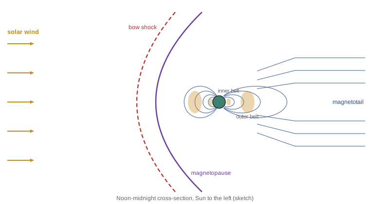
Because the solar wind is supersonic, and indeed faster than the speed of magnetic waves in it, a standing bow shock forms about 2 to 3 Earth radii upstream of the magnetopause, where the wind abruptly slows, heats and is deflected around the obstacle. The shocked plasma between the bow shock and the magnetopause is the magnetosheath. On the night side, the solar wind drags field lines into a long magnetotail, stretching hundreds of Earth radii downstream, with two lobes of nearly opposite field separated by a plasma sheet and its cross-tail current. The tail stores magnetic energy during periods of strong coupling and releases it suddenly in substorms, as lesson 11 describes.

Inside the magnetosphere, the plasma is organized by the field into several populations: the plasmasphere, a dense, cold torus of ionospheric plasma corotating with the Earth out to about 4 to 5 Earth radii; the ring current of energetic ions drifting around the Earth at 3 to 6 Earth radii, whose strength is measured by the Dst index; and the radiation belts.

Charged particle motion

A particle of charge \(q\), mass \(m\) and momentum \(p\) in a magnetic field gyrates around the field line at the cyclotron frequency \(\omega_c = qB/\gamma m\), with gyroradius \(r_g = p_\perp/qB\), where \(p_\perp = p\sin\alpha\) and \(\alpha\) is the pitch angle between the velocity and the field. A magnetic field does no work, so the particle's speed is constant. When the field varies slowly in space compared with the gyroradius, the particle's motion separates into three periodic motions on very different time scales, each associated with an adiabatic invariant.

First, gyration conserves the magnetic moment \(\mu = p_\perp^2/2mB\), equivalently \(\sin^2\alpha/B\). As a particle moves along a field line into a stronger field near the Earth, its perpendicular momentum must grow and, with the speed fixed, its parallel momentum shrinks. At the point where \(\sin^2\alpha = 1\), that is, where \(B_m = B_{eq}/\sin^2\alpha_{eq}\), it reverses: it is mirrored. Particles therefore bounce back and forth between mirror points in the northern and southern hemispheres. A particle whose mirror point lies below about 100 km collides with the atmosphere and is lost; the range of equatorial pitch angles that leads to loss is the loss cone, a few degrees wide at \(L = 4\).

Second, bouncing conserves the longitudinal invariant. The bounce period is approximately

Third, the field's gradient and curvature make the guiding center drift around the Earth, ions westward and electrons eastward, conserving the flux enclosed by the drift orbit. For an equatorially mirroring particle the gradient drift alone gives an angular drift rate \(3pvL/(2qB_0R_E^2)\), so the drift period is

Opposite drifts of ions and electrons carry a net westward current around the Earth: the ring current. During a storm it grows, its magnetic field opposes the Earth's at the equator, and ground magnetometers see the horizontal field drop by tens to hundreds of nanotesla; that drop is the Dst index.

The Boris pusher

The program integrates the motion of a 10 MeV proton at \(L = 4\) with the Boris algorithm, the standard method for charged particles in electromagnetic fields since its introduction by Jay Boris in 1970. Each step rotates the momentum vector about the local field by the exact angle appropriate to the time step, so the speed is conserved to rounding error no matter how many gyrations are followed, which ordinary Runge–Kutta methods cannot do. With 40 steps per gyration, the simulation follows the proton for 75 seconds, about 540 gyrations and 35 bounces.

The results check the theory. The gyroradius at 90° pitch angle is 955 km, small compared with the 25 000 km radius of the \(L = 4\) shell, so the adiabatic approximation applies. For an equatorially mirroring proton, the drift period from the orbit is 63 s against 66 s from the gradient-drift formula. For a 40° pitch angle, the bounce period is 2.14 s against 2.21 s from the approximate formula, and the mirror latitude is 24° from the orbit against 26° from \(B_m = B_{eq}/\sin^2\alpha\); the difference is mostly the gyroradius, since the code records the particle's position, not its guiding center, and 955 km at 25 000 km is about 2°. The 40° particle drifts more slowly, in 70 s, because it spends time at higher latitudes where the drift is weaker. The speed is conserved to \(10^{-14}\), confirming that the magnetic force does no work.

The radiation belts

Van Allen's instruments on Explorer 1 in 1958 saturated in a region of intense radiation, which he interpreted correctly as trapped particles; Explorer 3 and later Pioneer 3 mapped two belts. The inner belt, at about 1.2 to 2.5 Earth radii, holds energetic protons of tens to hundreds of MeV, produced mainly by the decay of neutrons knocked out of the atmosphere by cosmic rays. It is stable over years. The outer belt, at about 3 to 7 Earth radii, is dominated by electrons of hundreds of keV to several MeV and is highly variable: it can be emptied in hours during the main phase of a storm and refilled to higher intensity days later, through acceleration by waves and radial diffusion. NASA's twin Van Allen Probes, from 2012 to 2019, discovered that a third, temporary belt can form after some storms. The relatively empty region between the belts, the slot, is kept clear by scattering from radio waves in the plasmasphere.

The belts matter because they damage satellites and endanger astronauts. Energetic electrons penetrate spacecraft and deposit charge in insulators until it discharges, and energetic protons cause single-event upsets in electronics and degrade solar cells. Global navigation satellites orbit in the outer belt at about 4 Earth radii, and geostationary satellites at its outer edge; both are designed to tolerate its radiation. The International Space Station, at about 400 km, stays below the belts except where it crosses the South Atlantic Anomaly.