Waveguides and transmission lines

Plane waves spread through all of space. Guided waves are confined by conductors and carried from one place to another: from a transmitter to an antenna, from a magnetron to the cooking cavity of a microwave oven, from a telescope's receiver to its electronics. This lesson solves Maxwell's equations inside a hollow rectangular metal pipe, finds its transverse electric and transverse magnetic modes and their cutoff frequencies, and shows that guided waves have a phase velocity above \(c\) and a group velocity below it. It then treats the transmission line, a pair of conductors that carries a transverse electromagnetic wave at any frequency, and develops the circuit tools engineers use for it: characteristic impedance, reflection coefficient, standing-wave ratio and impedance matching.

Waves between conducting walls

Consider a wave traveling along the \(z\) axis inside a hollow tube with perfectly conducting walls. Inside the conductor the fields vanish, so at the inner surface the boundary conditions of lesson 4 require \(\mathbf{E}^{\parallel} = \mathbf{0}\) and \(B^{\perp} = 0\). We look for fields of the form \(\tilde{\mathbf{E}}(x, y)e^{i(kz - \omega t)}\) and similarly for \(\tilde{\mathbf{B}}\). Substituting into Maxwell's equations in vacuum shows that all the transverse components are fixed by the longitudinal components \(E_z\) and \(B_z\), which each satisfy

Unlike a plane wave, a guided wave cannot in general be purely transverse. Modes with \(E_z = 0\) are called transverse electric, TE; modes with \(B_z = 0\) are transverse magnetic, TM. A mode with both \(E_z\) and \(B_z\) zero, a TEM mode, is impossible in a hollow pipe: its transverse fields would satisfy the static equations in the cross-section, and with a single connected conductor around the boundary the only static solution is zero. TEM waves need two separate conductors, as in a coaxial cable.

The rectangular waveguide

Take a rectangular guide with inner width \(a\) along \(x\) and height \(b\) along \(y\), with \(a \geq b\). For TE modes, separation of variables, exactly as for Laplace's equation in PHYS-381, gives \(B_z = B_0\cos(m\pi x/a)\cos(n\pi y/b)\), where the cosines are chosen so that the derived transverse \(\mathbf{E}\) satisfies \(E^{\parallel} = 0\) on the walls. Substituting into the equation above gives the dispersion relation

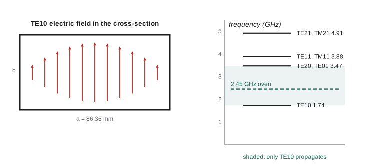
This is the \(\text{TE}_{mn}\) mode. If \(\omega\) is below the cutoff frequency \(\omega_{mn}\), the wave number is imaginary and the mode decays exponentially along the guide instead of propagating; it is evanescent. The lowest cutoff belongs to \(\text{TE}_{10}\), with \(\omega_{10} = c\pi/a\), corresponding to a free-space wavelength of \(2a\): the guide must be at least half a wavelength wide. TM modes need \(E_z\) to vanish on the walls, so they use sines, \(E_z = E_0\sin(m\pi x/a)\sin(n\pi y/b)\), and require both \(m\) and \(n\) to be at least 1; the lowest is \(\text{TM}_{11}\), with the same cutoff as \(\text{TE}_{11}\). Between the first and second cutoffs only the \(\text{TE}_{10}\) mode can travel, and guides are normally used in that single-mode band so that the energy is carried in one predictable pattern.

In the \(\text{TE}_{10}\) mode the electric field points across the narrow dimension, along \(y\), with strength varying as \(\sin(\pi x/a)\): zero at the side walls and largest in the middle. The magnetic field forms closed loops in the \(xz\) plane. The mode has a simple interpretation: it is a plane wave bouncing back and forth between the two side walls at an angle, zigzagging down the guide. The angle is fixed by the condition that the wave and its reflection interfere to give zero field at both walls. At the cutoff frequency the wave bounces straight across and makes no progress; far above cutoff it travels nearly straight down the guide.

Phase and group velocity in a guide

The phase velocity of a guided mode is \(v_p = \omega/k = c/\sqrt{1 - (\omega_{mn}/\omega)^2}\), greater than \(c\); the group velocity is \(v_g = d\omega/dk = c\sqrt{1 - (\omega_{mn}/\omega)^2}\), less than \(c\); and \(v_pv_g = c^2\), exactly the relation found for a plasma in lesson 8. The zigzag picture explains both. A plane wave moving at \(c\) at angle \(\theta\) to the axis has its crests sweeping along the axis faster than \(c\), as the point where ocean waves meet a beach runs along the beach faster than the waves themselves, while the energy, traveling at \(c\) along the zigzag, advances along the axis only at \(c\cos\theta\). The guide wavelength \(2\pi/k\) is longer than the free-space wavelength.

A microwave oven's magnetron produces about a kilowatt at 2.45 GHz and feeds it into the cooking cavity through a short rectangular guide, commonly of the standard WR-340 size, 86.36 mm by 43.18 mm. The program finds its lowest cutoffs and confirms that at 2.45 GHz only \(\text{TE}_{10}\) propagates, with a guide wavelength of about 17 cm. Waveguides carry the high-power signals of radar transmitters and particle accelerators, where their low loss matters: the fields touch only the walls, and the surface resistance of lesson 8 sets the attenuation. Rectangular and circular guides, and the dielectric guides that became optical fibers, were analyzed in the 1930s, though Lord Rayleigh had already shown in 1897 that hollow pipes could carry electromagnetic waves above a cutoff frequency.

Transmission lines

Two conductors, such as the inner and outer conductors of a coaxial cable or the two wires of a twisted pair, can carry a TEM wave at any frequency, down to direct current. For such a wave the transverse fields at each position along the line are exactly the static fields of the two conductors carrying charge \(\pm\lambda\) per unit length and current \(\pm I\). This lets the line be described by its static capacitance \(\mathcal{C}\) and inductance \(\mathcal{L}\) per unit length. Consider a short length \(dz\). The voltage drop along it is set by the inductance, and the current change by the charge that accumulates on the capacitance:

These are the telegrapher's equations, derived by Heaviside in the 1880s to explain how signals distort on long telegraph cables. Eliminating \(I\) gives a wave equation for \(V\) with speed \(v = 1/\sqrt{\mathcal{L}\mathcal{C}}\), and the ratio of voltage to current in a single traveling wave is the characteristic impedance

For a coaxial cable with inner radius \(a\), outer radius \(b\) and a dielectric of permittivity \(\varepsilon\), PHYS-381 gave \(\mathcal{C} = 2\pi\varepsilon/\ln(b/a)\) and the magnetostatics lessons give \(\mathcal{L} = (\mu_0/2\pi)\ln(b/a)\). Then \(v = 1/\sqrt{\mu_0\varepsilon} = c/n\), independent of the geometry, and \(Z_0 = (Z_{\text{vac}}/2\pi n)\ln(b/a)\). Common laboratory and radio cables are built for 50 \(\Omega\) and television cables for 75 \(\Omega\). The characteristic impedance is not a resistance: an ideal lossless line dissipates nothing. It is the ratio \(V/I\) the line presents to a wave traveling along it, set by the geometry.

Reflections, standing waves and matching

When a wave traveling along a line of impedance \(Z_0\) reaches a load \(Z_L\), the load forces the ratio \(V/I = Z_L\) at its terminals. A single forward wave has \(V/I = Z_0\), so unless \(Z_L = Z_0\) a reflected wave must arise, with amplitude ratio

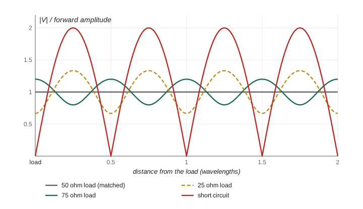
A matched load, \(Z_L = Z_0\), absorbs everything. A short circuit gives \(\Gamma = -1\) and an open circuit \(\Gamma = +1\): total reflection. This is the same structure as the Fresnel coefficient at normal incidence, \((n_1 - n_2)/(n_1 + n_2)\), because impedances of media scale as \(1/n\). The forward and reflected waves interfere to give a standing-wave pattern along the line, with maxima of \(|V|\) equal to \(1 + |\Gamma|\) and minima of \(1 - |\Gamma|\) times the forward amplitude, half a wavelength apart. Their ratio is the voltage standing-wave ratio, \(\text{VSWR} = (1 + |\Gamma|)/(1 - |\Gamma|)\), which engineers measure to judge how well a load is matched; the fraction of power delivered is \(1 - |\Gamma|^2\).

The impedance seen looking into a line of length \(l\) terminated by \(Z_L\) is \(Z_{\text{in}} = Z_0(Z_L + iZ_0\tan\beta l)/(Z_0 + iZ_L\tan\beta l)\), with \(\beta = 2\pi/\lambda\) on the line. A quarter-wavelength section is special: \(\tan\beta l\) is infinite, so \(Z_{\text{in}} = Z_0^2/Z_L\). A quarter-wave section of impedance \(\sqrt{Z_1Z_2}\) therefore matches \(Z_2\) to \(Z_1\), the transmission-line version of an antireflection coating. The match works exactly only at one frequency; the program shows how it degrades when the section is 20% too short or too long.

import math, cmath
c = 2.99792458e8; mu0 = 4e-7 * math.pi; eps0 = 8.8541878188e-12

# 1. Rectangular waveguide WR-340 (86.36 mm x 43.18 mm), used to feed microwave ovens
a, b = 86.36e-3, 43.18e-3
modes = []
for m in range(0, 4):
    for n in range(0, 4):
        if m == 0 and n == 0: continue
        fc = c / 2 * math.sqrt((m / a) ** 2 + (n / b) ** 2)
        kinds = ["TE"] if (m == 0 or n == 0) else ["TE", "TM"]
        for kd in kinds: modes.append((fc, f"{kd}{m}{n}"))
modes.sort()
print("lowest modes: " + ", ".join(f"{nm} {fc / 1e9:.3f} GHz" for fc, nm in modes[:6]))
f = 2.45e9; w = 2 * math.pi * f
fc10 = c / (2 * a)
vp = c / math.sqrt(1 - (fc10 / f) ** 2); vg = c * math.sqrt(1 - (fc10 / f) ** 2)
lam0 = c / f; lamg = lam0 / math.sqrt(1 - (fc10 / f) ** 2)
print(f"at 2.45 GHz only TE10 propagates: phase speed {vp / c:.3f} c, group speed {vg / c:.3f} c, "
      f"vp*vg = {vp * vg / c**2:.3f} c^2")
print(f"free-space wavelength {lam0 * 100:.2f} cm, guide wavelength {lamg * 100:.2f} cm")
# an evanescent mode: TE20 at 2.45 GHz
fc20 = c / a
kap = 2 * math.pi / c * math.sqrt(fc20 ** 2 - f ** 2)
print(f"TE20 (cutoff {fc20 / 1e9:.3f} GHz) decays by 1/e in {1 / kap * 1000:.1f} mm")

# 2. Coaxial line: characteristic impedance and speed from the geometry
ra, rb, er = 0.45e-3, 1.57e-3, 2.25         # inner and outer radius, polyethylene filling
Lp = mu0 / (2 * math.pi) * math.log(rb / ra); Cp = 2 * math.pi * er * eps0 / math.log(rb / ra)
Z0 = math.sqrt(Lp / Cp); v = 1 / math.sqrt(Lp * Cp)
print(f"coax: L' = {Lp * 1e9:.1f} nH/m, C' = {Cp * 1e12:.1f} pF/m, Z0 = {Z0:.1f} ohm, v = {v / c:.3f} c")

# 3. Reflection coefficient, standing-wave ratio and the fraction of power delivered
for ZL in (50.0, 75.0, 25.0, 0.0, 1e12, complex(50, 50)):
    G = (ZL - 50) / (ZL + 50)
    vswr = f"{(1 + abs(G)) / (1 - abs(G)):.2f}" if abs(G) < 0.999 else "infinite"
    tag = "open circuit" if abs(ZL) > 1e9 else ("short circuit" if ZL == 0 else (f"{ZL:.0f} ohm" if isinstance(ZL, float) else "50+50j ohm"))
    print(f"load {tag:>13s}: |Gamma| = {abs(G):.3f}, VSWR = {vswr}, power delivered {1 - abs(G)**2:.3f}")

# 4. Quarter-wave transformer: match a 100 ohm load to a 50 ohm line
Zt = math.sqrt(50 * 100)
def zin(Z0l, ZL, beta_l):
    t = math.tan(beta_l)
    return Z0l * (ZL + 1j * Z0l * t) / (Z0l + 1j * ZL * t)
for frac in (0.25, 0.20, 0.30):
    Zi = zin(Zt, 100.0, 2 * math.pi * frac)
    G = (Zi - 50) / (Zi + 50)
    im = round(Zi.imag, 1) + 0.0
    print(f"section {Zt:.1f} ohm, length {frac:.2f} wavelength: Zin = {Zi.real:.1f} {'+' if im >= 0 else '-'} {abs(im):.1f}j ohm, |Gamma| = {abs(G):.3f}")

lowest modes: TE10 1.736 GHz, TE01 3.471 GHz, TE20 3.471 GHz, TE11 3.881 GHz, TM11 3.881 GHz, TE21 4.909 GHz
at 2.45 GHz only TE10 propagates: phase speed 1.417 c, group speed 0.706 c, vp*vg = 1.000 c^2
free-space wavelength 12.24 cm, guide wavelength 17.34 cm
TE20 (cutoff 3.471 GHz) decays by 1/e in 19.4 mm
coax: L' = 249.9 nH/m, C' = 100.2 pF/m, Z0 = 49.9 ohm, v = 0.667 c
load        50 ohm: |Gamma| = 0.000, VSWR = 1.00, power delivered 1.000
load        75 ohm: |Gamma| = 0.200, VSWR = 1.50, power delivered 0.960
load        25 ohm: |Gamma| = 0.333, VSWR = 2.00, power delivered 0.889
load short circuit: |Gamma| = 1.000, VSWR = infinite, power delivered 0.000
load  open circuit: |Gamma| = 1.000, VSWR = infinite, power delivered 0.000
load    50+50j ohm: |Gamma| = 0.447, VSWR = 2.62, power delivered 0.800
section 70.7 ohm, length 0.25 wavelength: Zin = 50.0 + 0.0j ohm, |Gamma| = 0.000
section 70.7 ohm, length 0.20 wavelength: Zin = 52.5 - 10.9j ohm, |Gamma| = 0.109
section 70.7 ohm, length 0.30 wavelength: Zin = 52.5 + 10.9j ohm, |Gamma| = 0.109

The WR-340 guide carries only \(\text{TE}_{10}\) at 2.45 GHz; the next modes, \(\text{TE}_{20}\) and \(\text{TE}_{01}\), cut off at 3.47 GHz, and below cutoff \(\text{TE}_{20}\) decays by a factor \(e\) within about 2 cm, so any field in that pattern dies out near its source. The phase and group speeds, 1.42c and 0.71c, multiply to exactly \(c^2\). The coaxial cable, with a polyethylene filling of \(\varepsilon_r = 2.25\) and a radius ratio of 3.49, comes out at about 50 \(\Omega\) and carries signals at two thirds of the speed of light, so a 1 m cable delays a signal by 5 ns, a fact every timing system must allow for. A 75 \(\Omega\) load on a 50 \(\Omega\) line reflects 4% of the power and has a VSWR of 1.5; a quarter-wave section of 70.7 \(\Omega\) matches a 100 \(\Omega\) load perfectly at its design frequency and still delivers about 99% of the power when its length is off by 20%.