Potentials, gauges and retarded potentials

Lessons 6 to 9 studied fields far from their sources. To find the fields that a given set of changing charges and currents produce, it is easier to work with potentials, as in statics. This lesson shows how the scalar potential \(V\) and vector potential \(\mathbf{A}\) are generalized to changing fields, explains the freedom to change them by a gauge transformation without altering any measurable field, and introduces the two common gauges. In the Lorenz gauge the potentials obey wave equations whose solutions are the retarded potentials: the potential at a point is built from the sources as they were when a light signal now arriving there left them. Applied to a moving point charge, this gives the Liénard–Wiechert potentials, which a program checks against relativity.

Potentials for changing fields

Because \(\nabla\cdot\mathbf{B} = 0\) still holds, we can still write \(\mathbf{B} = \nabla\times\mathbf{A}\). Faraday's law then reads \(\nabla\times(\mathbf{E} + \partial\mathbf{A}/\partial t) = \mathbf{0}\), so the combination in brackets is curl-free and can be written as minus the gradient of a scalar. Therefore

In statics the second term vanishes and \(\mathbf{E} = -\nabla V\) as before. Now the electric field has a part that comes from the changing vector potential, which is the induced field of Faraday's law. Writing the fields this way satisfies the two homogeneous Maxwell equations automatically. The other two become equations for the potentials:

Four unknown functions, \(V\) and the three components of \(\mathbf{A}\), now replace the six field components, and the equations are linear in the sources. But they look complicated, because \(V\) and \(\mathbf{A}\) are coupled. The next step simplifies them by using a freedom that the potentials have and the fields do not.

Gauge transformations

The potentials are not unique. If \(\lambda(\mathbf{r}, t)\) is any smooth function, the new potentials

give the same fields. The curl of a gradient vanishes, so \(\mathbf{B}\) is unchanged, and in \(\mathbf{E}\) the new terms \(+\nabla(\partial\lambda/\partial t) - \partial(\nabla\lambda)/\partial t\) cancel because the order of differentiation does not matter. Such a change is a gauge transformation, and the fact that the physics does not change is gauge invariance. In classical physics it is a convenience: we can choose \(\lambda\) to make the potentials satisfy an extra condition, a gauge, that simplifies the equations. In quantum mechanics it turns out to be much more, a principle from which the form of the electromagnetic interaction itself can be derived, and its generalizations underlie the whole Standard Model of particle physics. The program checks the cancellation numerically for a sample \(\lambda\).

The Coulomb gauge sets \(\nabla\cdot\mathbf{A} = 0\). Then the first potential equation becomes Poisson's equation, \(\nabla^2V = -\rho/\varepsilon_0\), whose solution is the familiar instantaneous Coulomb potential of the charge distribution at that same moment. That looks like a violation of causality, but it is not: \(V\) alone is not measurable, and the equation for \(\mathbf{A}\) in this gauge contains a compensating term that ensures \(\mathbf{E}\) responds only after a delay. The Coulomb gauge is useful in quantum optics and for separating radiation from static effects.

The Lorenz gauge, introduced by the Danish physicist Ludvig Lorenz in 1867, sets

It is often attributed to Hendrik Lorentz, the Dutch physicist after whom the Lorentz force and transformation are named, but Lorenz used it first. With this condition the bracket in the second potential equation vanishes, and both equations decouple into the same form:

Each potential obeys an inhomogeneous wave equation driven by its source, with the d'Alembertian \(\Box^2\) playing the role that the Laplacian plays in statics. The Lorenz condition treats \(V\) and \(\mathbf{A}\) on an equal footing, and the capstone shows that \((V/c, \mathbf{A})\) form a four-vector in relativity, which makes the Lorenz gauge the natural choice when relativity matters.

The retarded potentials

In statics the solution of \(\nabla^2V = -\rho/\varepsilon_0\) is \(V = \frac{1}{4\pi\varepsilon_0}\int\rho(\mathbf{r}')/\mathscr{r}\,d\tau'\). For changing sources the natural guess is to use the same formula but to evaluate each source at the retarded time

the moment when a signal traveling at \(c\) must have left the source point \(\mathbf{r}'\) in order to reach the field point \(\mathbf{r}\) at time \(t\). The retarded potentials are

Direct differentiation shows that they satisfy the inhomogeneous wave equations and the Lorenz condition; the calculation is subtle because \(\mathscr{r}\) appears both in the denominator and inside the source's time argument, and the extra terms that arise conspire to cancel. The guess works for the potentials. It would not work for the fields: the retarded versions of Coulomb's and the Biot–Savart laws are wrong, and the correct expressions, known as Jefimenko's equations after Oleg Jefimenko who published them in 1966, contain extra terms involving the time derivatives of the sources. Those terms are what produce radiation.

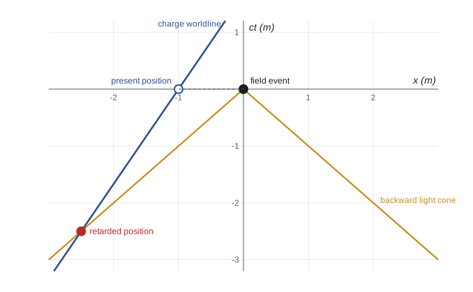
The wave equation also has advanced solutions, with \(t_a = t + \mathscr{r}/c\), in which effects precede their causes. They are mathematically valid but are excluded on physical grounds: we see sources as they were, never as they will be. The figure shows the retarded time on a spacetime diagram.

Two examples

First, a long straight wire whose current jumps from zero to \(I_0\) at \(t = 0\). In the Lorenz gauge the wire is neutral, so \(V = 0\), and at distance \(s\) the retarded integral for \(\mathbf{A}\) includes only the part of the wire close enough for a signal to have arrived: \(|z| \leq \sqrt{c^2t^2 - s^2}\). Integrating gives

Nothing happens until the news of the switch-on arrives at \(t = s/c\). Then an electric field appears, opposing the current, and dies away as \(1/t\), leaving the steady magnetic field \(\mu_0I_0/2\pi s\) of a long wire. The program differentiates \(\mathbf{A}\) numerically and compares with the formula.

Second, a point charge \(q\) moving along a known path. Its retarded potentials involve only the single retarded time at which its worldline crosses the backward light cone, but they carry an extra factor because a moving charge is effectively stretched or compressed in the integral. The result is the Liénard–Wiechert potentials, found by Alfred-Marie Liénard in 1898 and Emil Wiechert in 1900:

with \(\boldsymbol{\mathscr{r}}\) and \(\mathbf{v}\) evaluated at the retarded time. For a charge approaching the field point the denominator is smaller than \(\mathscr{r}c\) and the potential is enhanced. The program finds the retarded time numerically by bisection for a charge moving at \(0.8c\), and checks the Liénard–Wiechert potential against an independent route: the Coulomb potential in the charge's rest frame, Lorentz-transformed to the laboratory, which gives \(V = \gamma kq/\sqrt{\gamma^2(x - vt)^2 + y^2}\) in terms of the present position.

import math
c = 2.99792458e8; eps0 = 8.8541878188e-12; mu0 = 4e-7 * math.pi; k = 1 / (4 * math.pi * eps0)

# 1. Retarded time for a charge moving along x at constant speed v, passing x = 0 at t = 0.
#    Solve c (t - tr) = distance from the charge's position at tr to the field point, by bisection.
def retarded_time(t, xp, yp, v):
    f = lambda tr: c * (t - tr) - math.hypot(xp - v * tr, yp)
    lo, hi = t - 1.0, t          # f(lo) > 0, f(t) <= 0
    for _ in range(200):
        mid = 0.5 * (lo + hi)
        if f(mid) > 0: lo = mid
        else: hi = mid
    return 0.5 * (lo + hi)
q = 1e-9; v = 0.8 * c
xp, yp, t = 0.0, 1.0, 0.0          # field point 1 m from the path, at the moment the charge passes x = 0
tr = retarded_time(t, xp, yp, v)
xr = v * tr; sep = math.hypot(xp - xr, yp)
print(f"retarded time {tr * 1e9:.4f} ns, charge was at x = {xr:.4f} m, {sep:.4f} m away")
# Lienard-Wiechert scalar potential V = k q / (sep - sep_vec . v / c)
dot = ((xp - xr) * v) / c
V_lw = k * q / (sep - dot)
print(f"Lienard-Wiechert V = {V_lw:.3f} V; Coulomb with the present distance would give {k * q / math.hypot(xp, yp):.3f} V, "
      f"with the retarded distance {k * q / sep:.3f} V")
gamma = 1 / math.sqrt(1 - (v / c) ** 2)
# same potential from the Lorentz-transformed Coulomb potential: V = gamma k q / sqrt(gamma^2 (x - vt)^2 + y^2)
print(f"check from relativity: gamma k q / sqrt(gamma^2 (x - vt)^2 + y^2) = {gamma * k * q / math.hypot(gamma * (xp - v * t), yp):.3f} V")

# 2. A wire current switched on at t = 0 (I = I0 for t > 0): the vector potential at distance s is
#    A(s,t) = (mu0 I0 / 2pi) ln[(ct + sqrt(c^2 t^2 - s^2))/s] for ct > s, and zero before.
I0, s = 1.0, 3.0
def A(t):
    if c * t <= s: return 0.0
    return mu0 * I0 / (2 * math.pi) * math.log((c * t + math.sqrt((c * t) ** 2 - s * s)) / s)
for ct in (2.0, 3.5, 5.0, 30.0, 300.0):
    t = ct / c; h = t * 1e-6
    E_num = -(A(t + h) - A(t - h)) / (2 * h) + 0.0
    E_exact = 0.0 if ct <= s else -mu0 * I0 * c / (2 * math.pi * math.sqrt(ct * ct - s * s))
    print(f"ct = {ct:5.1f} m: A = {A(t) * 1e7:.4f} x 1e-7 T m, E = -dA/dt numeric {E_num:.4f} V/m, formula {E_exact:.4f} V/m")

# 3. Gauge freedom: A -> A + grad(lam), V -> V - dlam/dt leaves E = -grad V - dA/dt unchanged,
#    because the extra terms are d/dx(dlam/dt) - d/dt(dlam/dx). Check for lam = x^2 t^3 + sin(x t).
lam = lambda x, t: x * x * t ** 3 + math.sin(x * t)
hh = 1e-4
dlam_dt = lambda x, t: (lam(x, t + hh) - lam(x, t - hh)) / (2 * hh)
dlam_dx = lambda x, t: (lam(x + hh, t) - lam(x - hh, t)) / (2 * hh)
for x0, t0 in ((0.7, 0.3), (1.5, 2.0)):
    term1 = (dlam_dt(x0 + hh, t0) - dlam_dt(x0 - hh, t0)) / (2 * hh)    # from -grad(-dlam/dt)
    term2 = (dlam_dx(x0, t0 + hh) - dlam_dx(x0, t0 - hh)) / (2 * hh)    # from -d/dt(grad lam)
    print(f"at x = {x0}, t = {t0}: change in E_x = {term1:.6f} - {term2:.6f} = {term1 - term2:.1e}")

retarded time -5.5594 ns, charge was at x = -1.3333 m, 1.6667 m away
Lienard-Wiechert V = 14.979 V; Coulomb with the present distance would give 8.988 V, with the retarded distance 5.393 V
check from relativity: gamma k q / sqrt(gamma^2 (x - vt)^2 + y^2) = 14.979 V
ct =   2.0 m: A = 0.0000 x 1e-7 T m, E = -dA/dt numeric 0.0000 V/m, formula 0.0000 V/m
ct =   3.5 m: A = 1.1392 x 1e-7 T m, E = -dA/dt numeric -33.2590 V/m, formula -33.2590 V/m
ct =   5.0 m: A = 2.1972 x 1e-7 T m, E = -dA/dt numeric -14.9896 V/m, formula -14.9896 V/m
ct =  30.0 m: A = 5.9864 x 1e-7 T m, E = -dA/dt numeric -2.0087 V/m, formula -2.0087 V/m
ct = 300.0 m: A = 10.5966 x 1e-7 T m, E = -dA/dt numeric -0.1999 V/m, formula -0.1999 V/m
at x = 0.7, t = 0.3: change in E_x = 1.312254 - 1.312254 = 0.0e+00
at x = 1.5, t = 2.0: change in E_x = 34.586648 - 34.586648 = 0.0e+00

At the moment the charge passes closest to the field point, the light now arriving left it 5.56 ns earlier, when it was 1.33 m back along its path and 1.67 m away. The Liénard–Wiechert potential is 14.98 V, larger than the naive Coulomb value for either the present or the retarded distance, and it agrees exactly with the Lorentz-transformed Coulomb potential. The agreement is a first sign of the capstone's message: the retarded potentials of Maxwell's theory already contain special relativity. For the switched-on wire, nothing happens until \(ct = 3\) m, then the field jumps in and fades, with the numerical derivative matching the formula at every time. The gauge check confirms that the two extra terms in \(\mathbf{E}\) cancel at any point, to the precision of the arithmetic.