Maxwell's equations in vacuum and in matter, and boundary conditions

With Faraday's law and the displacement current in place, the four Maxwell equations are complete. This lesson collects them, reads each one physically, and rewrites them for materials, where bound charges and currents are handled by the auxiliary fields \(\mathbf{D}\) and \(\mathbf{H}\) introduced in PHYS-381. It then derives the boundary conditions that link the fields on the two sides of any surface, the tool that lessons 7 to 9 use for reflection, refraction and waveguides. A short program checks the vacuum equations on a plane wave by finite differences and shows how field lines bend at dielectric and magnetic surfaces.

The equations in vacuum

In vacuum, with charge density \(\rho\) and current density \(\mathbf{J}\) as sources,

Together with the Lorentz force law they form a closed theory: given the charges and currents, the equations determine the fields, and given the fields, the force law determines how the charges move. A few structural features are worth noting. The equations are first-order partial differential equations for six field components. Charge conservation is not an extra assumption but a consequence, as lesson 1 showed by taking the divergence of (iv). The divergence equations (i) and (ii) are, in a sense, constraints on initial conditions: if they hold at one moment, the curl equations guarantee they hold later. And the equations are nearly symmetric between \(\mathbf{E}\) and \(\mathbf{B}\). In empty space, where \(\rho\) and \(\mathbf{J}\) vanish, the replacement \(\mathbf{E} \to c\mathbf{B}\), \(c\mathbf{B} \to -\mathbf{E}\) maps the set into itself.

The asymmetry that remains comes from the sources: there are electric charges but, as far as any experiment has found, no magnetic charges. If magnetic monopoles existed, (ii) would acquire a magnetic charge density and (iii) a magnetic current, and the symmetry would be complete. Paul Dirac showed in 1931 that the existence of even one monopole anywhere in the universe would explain why electric charge comes in discrete units. Searches continue, at accelerators and in cosmic rays, so far without success.

The integral forms

Each equation has an integral form obtained from the divergence theorem or Stokes' theorem. For any closed surface \(S\) enclosing volume \(V\), and any surface \(S\) bounded by a closed loop \(P\),

These are the forms used for problems with symmetry and, below, for deriving boundary conditions. The differential and integral forms say the same thing; the differential forms are local and are the ones that lead to wave equations.

Maxwell's equations in matter

Inside materials the charges and currents divide into free ones, which we control, and bound ones, which the material produces in response to the fields. PHYS-381 showed that a polarization \(\mathbf{P}\) produces bound charge \(\rho_b = -\nabla\cdot\mathbf{P}\), and a magnetization \(\mathbf{M}\) produces bound current \(\mathbf{J}_b = \nabla\times\mathbf{M}\). When fields change, there is one more piece. A changing polarization moves bound charge, which is a current: if \(\mathbf{P}\) changes, the bound charge on the faces of a small block changes, and the current needed to carry it is

This polarization current satisfies its own continuity equation with the bound charge, \(\nabla\cdot\mathbf{J}_p = \partial(\nabla\cdot\mathbf{P})/\partial t = -\partial\rho_b/\partial t\), as it must. It has nothing to do with magnetization currents, which carry no net charge anywhere. The total charge and current densities are therefore \(\rho = \rho_f - \nabla\cdot\mathbf{P}\) and \(\mathbf{J} = \mathbf{J}_f + \nabla\times\mathbf{M} + \partial\mathbf{P}/\partial t\). Putting these into Maxwell's equations and collecting terms with \(\mathbf{D} = \varepsilon_0\mathbf{E} + \mathbf{P}\) and \(\mathbf{H} = \mathbf{B}/\mu_0 - \mathbf{M}\) gives

In this form the displacement current is \(\partial\mathbf{D}/\partial t\), which includes both the vacuum term \(\varepsilon_0\,\partial\mathbf{E}/\partial t\) and the polarization current. Maxwell's name for it came from his picture of a dielectric, in which the ether itself was polarized and its charges were displaced. These equations are not complete until we say how \(\mathbf{D}\) and \(\mathbf{H}\) depend on \(\mathbf{E}\) and \(\mathbf{B}\). For linear, isotropic media the constitutive relations are

with \(\varepsilon = \varepsilon_r\varepsilon_0\) and \(\mu = \mu_r\mu_0\). These relations are good approximations for many materials but by no means all: ferromagnets are nonlinear and hysteretic, crystals are anisotropic so that \(\varepsilon\) becomes a tensor, and at high frequencies \(\varepsilon\) depends on frequency, an effect called dispersion that lesson 8 develops. The macroscopic fields are averages over many atoms; at the scale of individual atoms the vacuum equations with all charges counted are the correct description.

Boundary conditions

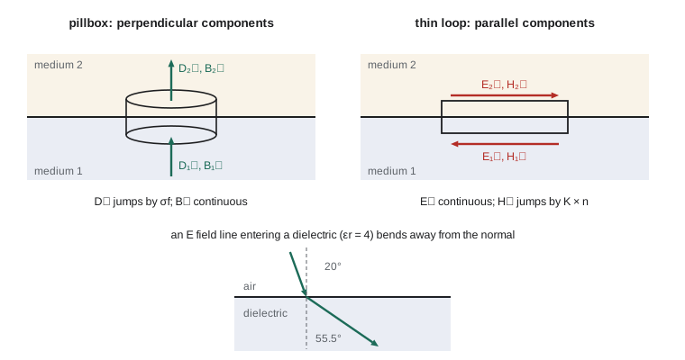
At the surface between two media, or at a sheet of surface charge or current, the fields can change abruptly. The integral forms fix how. Let \(\hat{\mathbf{n}}\) be the unit normal pointing from medium 1 into medium 2, \(\sigma_f\) the free surface charge and \(\mathbf{K}_f\) the free surface current. Apply the two divergence equations to a thin pillbox straddling the surface. As its thickness shrinks to zero, only the flux through the top and bottom faces survives, giving

Now apply the two curl equations to a thin rectangular loop straddling the surface. As its height shrinks, the flux of \(\partial\mathbf{B}/\partial t\) or \(\partial\mathbf{D}/\partial t\) through it vanishes, because those fields are finite and the area goes to zero. Only a genuine surface current, an infinitely thin sheet, can contribute to the enclosed current. The result is

These four conditions hold for any fields, static or changing. They say that the parallel component of \(\mathbf{E}\) and the perpendicular component of \(\mathbf{B}\) are always continuous, the perpendicular component of \(\mathbf{D}\) jumps by the free surface charge, and the parallel component of \(\mathbf{H}\) jumps by the free surface current. For linear media without free charge or current at the surface they become \(\varepsilon_1E_1^{\perp} = \varepsilon_2E_2^{\perp}\), \(\mathbf{E}_1^{\parallel} = \mathbf{E}_2^{\parallel}\), \(B_1^{\perp} = B_2^{\perp}\) and \(\mathbf{B}_1^{\parallel}/\mu_1 = \mathbf{B}_2^{\parallel}/\mu_2\). For a perfect conductor, where the fields inside vanish, the parallel component of \(\mathbf{E}\) and the perpendicular component of \(\mathbf{B}\) just outside must be zero; the surface charge and current then adjust themselves to whatever the outside fields require.

Checking the equations and bending field lines

The program below does two things. It takes the plane wave \(\mathbf{E} = E_0\cos(kz - \omega t)\,\hat{\mathbf{x}}\), \(\mathbf{B} = (E_0/c)\cos(kz - \omega t)\,\hat{\mathbf{y}}\) with \(\omega = ck\), the subject of lesson 6, and evaluates every derivative in the four vacuum equations by central differences at an arbitrary point and time. It then applies the boundary conditions to a field crossing from air into a dielectric with \(\varepsilon_r = 4\), and to a magnetic field leaving iron with \(\mu_r = 1000\). With no free surface charge, continuity of \(E^{\parallel}\) and of \(\varepsilon E^{\perp}\) gives the refraction law for field lines,

where the angles are measured from the normal. The magnetic analog replaces \(\varepsilon\) by \(\mu\).

import math
eps0 = 8.8541878188e-12; mu0 = 1.25663706212e-6; c = 1 / math.sqrt(eps0 * mu0)

# 1. Check all four vacuum Maxwell equations, by finite differences, for the plane wave
#    E = E0 cos(kz - wt) x-hat,  B = (E0/c) cos(kz - wt) y-hat
E0, lam = 100.0, 0.5
k = 2 * math.pi / lam; w = c * k
def E(x, y, z, t): return (E0 * math.cos(k * z - w * t), 0.0, 0.0)
def B(x, y, z, t): return (0.0, E0 / c * math.cos(k * z - w * t), 0.0)
def d(f, comp, axis, p, h):
    q1 = list(p); q2 = list(p); q1[axis] += h; q2[axis] -= h
    return (f(*q1)[comp] - f(*q2)[comp]) / (2 * h)
p = (0.1, 0.2, 0.13, 2e-10); h = 1e-6; ht = h / c
divE = sum(d(E, i, i, p, h) for i in range(3))
divB = sum(d(B, i, i, p, h) for i in range(3))
def curl(f, p):
    return (d(f, 2, 1, p, h) - d(f, 1, 2, p, h), d(f, 0, 2, p, h) - d(f, 2, 0, p, h), d(f, 1, 0, p, h) - d(f, 0, 1, p, h))
cE, cB = curl(E, p), curl(B, p)
dBdt = [d(B, i, 3, p, ht) for i in range(3)]
dEdt = [d(E, i, 3, p, ht) for i in range(3)]
print(f"div E = {divE:.2e}, div B = {divB:.2e}")
print(f"curl E (y) = {cE[1]:.4f},  -dB/dt (y) = {-dBdt[1]:.4f}")
print(f"curl B (x) = {cB[0]:.4e}, mu0 eps0 dE/dt (x) = {mu0 * eps0 * dEdt[0]:.4e}")

# 2. Boundary conditions at a dielectric interface (no free surface charge):
#    E parallel and D perpendicular are continuous, so tan(theta2)/tan(theta1) = er2/er1
er1, er2 = 1.0, 4.0
for th1 in (20, 45, 70):
    t1 = math.radians(th1)
    Epar, Eperp1 = math.sin(t1), math.cos(t1)          # field of unit strength in medium 1
    Eperp2 = er1 / er2 * Eperp1                          # D perpendicular continuous
    th2 = math.degrees(math.atan2(Epar, Eperp2))
    print(f"E line at {th1} deg from the normal in air bends to {th2:.1f} deg in er = 4; |E2|/|E1| = {math.hypot(Epar, Eperp2):.3f}")

# 3. Magnetic version: B perpendicular and H parallel continuous at an iron surface (mur = 1000)
mur = 1000.0
for th_iron in (60.0, 85.0, 89.9):
    t = math.radians(th_iron)
    Bperp, Bpar_iron = math.cos(t), math.sin(t)
    Bpar_air = Bpar_iron / mur
    print(f"B line at {th_iron} deg from the normal inside iron leaves at {math.degrees(math.atan2(Bpar_air, Bperp)):.3f} deg in air")

div E = 0.00e+00, div B = 0.00e+00
curl E (y) = -968.6732,  -dB/dt (y) = -968.6732
curl B (x) = 3.2311e-06, mu0 eps0 dE/dt (x) = 3.2311e-06
E line at 20 deg from the normal in air bends to 55.5 deg in er = 4; |E2|/|E1| = 0.415
E line at 45 deg from the normal in air bends to 76.0 deg in er = 4; |E2|/|E1| = 0.729
E line at 70 deg from the normal in air bends to 84.8 deg in er = 4; |E2|/|E1| = 0.944
B line at 60.0 deg from the normal inside iron leaves at 0.099 deg in air
B line at 85.0 deg from the normal inside iron leaves at 0.655 deg in air
B line at 89.9 deg from the normal inside iron leaves at 29.811 deg in air

Both divergences vanish identically, and the curl of each field matches the time derivative of the other to all printed digits. Notably, \(\nabla\times\mathbf{B}\) equals \(\mu_0\varepsilon_0\,\partial\mathbf{E}/\partial t\) only because \(\omega = ck\); with any other ratio the wave would fail to satisfy the equations, which is the first hint that Maxwell's equations fix the speed of light. In the dielectric, field lines bend away from the normal and the field is weakened, most strongly for nearly normal incidence where \(E^{\perp}\) dominates. The iron example shows why magnetic field lines leave the surface of a high-permeability material almost exactly perpendicular to it: even a line running at 85° to the normal inside the iron emerges within a degree of the normal. Only a line running almost parallel to the surface inside, at 89.9°, leaves at an appreciable angle. This is why iron pole pieces are used to shape fields in motors and magnetic resonance scanners: the shape of the iron surface fixes the direction of the field just outside it.