The formalism: Hilbert space, Hermitian operators and eigenvectors

Lessons 2 to 7 solved one problem after another with the same moves: find the eigenfunctions of the Hamiltonian, check that they are orthonormal, expand the initial state in them by projection, and attach time-dependent phases. Those moves work for a reason. Wave functions are vectors, observables are linear operators on those vectors, and the special properties that kept appearing, real energies, orthogonal eigenfunctions, complete sets, follow from one property of the operators: they are Hermitian. This lesson sets out that structure, which John von Neumann axiomatized in his 1932 book on the mathematical foundations of quantum mechanics and which Paul Dirac's 1930 textbook expressed in the bra-ket notation physicists still use. The payoff is that every system, spins and atoms and fields alike, is handled by the same linear algebra.

Wave functions as vectors

A vector space is a set of objects that can be added and multiplied by numbers, with the usual rules. The square-integrable functions on the line form one, over the complex numbers: if \(f\) and \(g\) are square-integrable, so is \(af + bg\). The inner product of two functions generalizes the dot product:

It is linear in the second argument, conjugate-linear in the first, satisfies \(\langle g|f\rangle = \langle f|g\rangle^{*}\), and gives a length, the norm \(\|f\| = \sqrt{\langle f|f\rangle}\), which is zero only for the zero function. The Schwarz inequality \(|\langle f|g\rangle|^2 \leq \langle f|f\rangle\langle g|g\rangle\), which follows from requiring \(\|f - \lambda g\|^2 \geq 0\) for the best choice of \(\lambda\), guarantees that the inner product of two square-integrable functions is finite. A space of this kind that is also complete, meaning that every Cauchy sequence of vectors converges to a vector in the space, is a Hilbert space, after David Hilbert, whose work on integral equations between 1904 and 1910 laid the groundwork. MATH-445 develops the theory; here we use it.

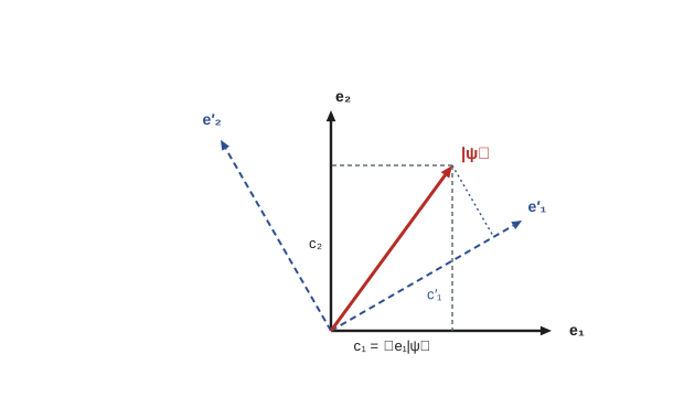
Physical states are normalized vectors, \(\langle\psi|\psi\rangle = 1\), with the understanding that \(\psi\) and \(e^{i\alpha}\psi\) represent the same state. Two functions are orthogonal if \(\langle f|g\rangle = 0\). A set \(\{e_n\}\) is orthonormal if \(\langle e_m|e_n\rangle = \delta_{mn}\) and complete if every vector can be expanded in it, \(\psi = \sum c_ne_n\) with \(c_n = \langle e_n|\psi\rangle\). The sine functions of the infinite well, the Hermite functions of the oscillator, and, for spin, the two vectors \(|{\uparrow}\rangle\) and \(|{\downarrow}\rangle\), are all orthonormal bases of their spaces. In any orthonormal basis, a state is represented by its list of components \(c_n\), and the inner product becomes \(\langle f|g\rangle = \sum_n f_n^{*}g_n\), exactly as for vectors in three dimensions.

Dirac notation

Dirac wrote a state as a ket \(|\psi\rangle\) and the operation of taking its inner product with something as a bra \(\langle\psi|\). Putting them together makes a bracket, \(\langle\phi|\psi\rangle\). The notation is economical because it does not commit to a basis: \(|\psi\rangle\) is the abstract vector, and \(\psi(x)\), the wave function, is its set of components in the position basis. In the energy basis of a system with eigenstates \(|n\rangle\), the same state has components \(c_n = \langle n|\psi\rangle\), and in the momentum basis it has components \(\Phi(p) = \langle p|\psi\rangle\), the momentum-space wave function of lesson 6. These are three descriptions of one vector, as a velocity can be described by components along any set of axes.

Completeness of an orthonormal basis can be written compactly as the resolution of the identity,

meaning that \(\sum_n|n\rangle\langle n|\psi\rangle = |\psi\rangle\) for every state. Each term \(\hat P_n = |n\rangle\langle n|\) is a projection operator, which picks out the component of a vector along \(|n\rangle\). Inserting the identity in this form is the most useful trick in quantum calculations; it converts any abstract expression into sums over components.

Operators and matrices

A linear operator \(\hat Q\) maps vectors to vectors and respects superposition: \(\hat Q(a|f\rangle + b|g\rangle) = a\hat Q|f\rangle + b\hat Q|g\rangle\). Position \(\hat x\), momentum \(\hat p = -i\hbar\,d/dx\), the Hamiltonian, the ladder operators of lesson 5: all are linear. In an orthonormal basis an operator is represented by a matrix,

so applying the operator becomes multiplying the column of components by the matrix. In its own eigenbasis the Hamiltonian is diagonal, \(H_{mn} = E_n\delta_{mn}\). For the oscillator, the ladder operators have entries only next to the diagonal, \(\langle n + 1|\hat a_+|n\rangle = \sqrt{n + 1}\), and so do \(\hat x\) and \(\hat p\). This is the matrix mechanics that Werner Heisenberg discovered in June 1925 on the island of Heligoland and that Max Born and Pascual Jordan recognized as matrix algebra a few weeks later. Schrödinger showed in 1926 that his wave mechanics and their matrix mechanics give identical results; the formalism of this lesson makes the equivalence obvious, since they are the same operators written in different bases.

Hermitian operators

The Hermitian conjugate \(\hat Q^{\dagger}\) of an operator is defined by \(\langle f|\hat Q^{\dagger}g\rangle = \langle\hat Qf|g\rangle\) for all \(f\) and \(g\); in matrix form it is the conjugate transpose. An operator is Hermitian if \(\hat Q^{\dagger} = \hat Q\), that is,

The connection to physics is this: the expectation value of an observable must be real, since it is the average of real measurement results, and \(\langle Q\rangle = \langle\psi|\hat Q\psi\rangle\) is real for every \(\psi\) if and only if \(\hat Q\) is Hermitian. (One direction is immediate: \(\langle\psi|\hat Q\psi\rangle^{*} = \langle\hat Q\psi|\psi\rangle = \langle\psi|\hat Q\psi\rangle\). For the other, apply the reality condition to \(f + g\) and \(f + ig\).) So observables are represented by Hermitian operators. Position is Hermitian trivially, since \(x\) is real. Momentum is Hermitian because of an integration by parts:

the boundary term vanishing for normalizable functions. The factor \(-i\) is essential: \(d/dx\) alone is anti-Hermitian, and multiplying by \(i\) fixes that. The Hamiltonian, a sum of \(\hat p^2/2m\) and a real \(V(x)\), is Hermitian too. Products of Hermitian operators need not be: \((\hat A\hat B)^{\dagger} = \hat B\hat A\), which equals \(\hat A\hat B\) only if they commute. That is why \(\hat x\hat p\) is not Hermitian but \((\hat x\hat p + \hat p\hat x)/2\) is.

The two key theorems

Hermitian operators have eigenvalues and eigenvectors with exactly the properties we have been relying on.

Theorem 1: the eigenvalues of a Hermitian operator are real. Suppose \(\hat Q|q\rangle = q|q\rangle\) with \(|q\rangle \neq 0\). Then \(\langle q|\hat Qq\rangle = q\langle q|q\rangle\), while \(\langle\hat Qq|q\rangle = q^{*}\langle q|q\rangle\). Hermiticity makes these equal, and \(\langle q|q\rangle > 0\), so \(q = q^{*}\).

Theorem 2: eigenvectors belonging to different eigenvalues are orthogonal. Let \(\hat Q|q\rangle = q|q\rangle\) and \(\hat Q|q'\rangle = q'|q'\rangle\) with \(q \neq q'\). Then \(\langle q'|\hat Qq\rangle = q\langle q'|q\rangle\) and \(\langle\hat Qq'|q\rangle = q'^{*}\langle q'|q\rangle = q'\langle q'|q\rangle\), using theorem 1. Hermiticity equates them, so \((q - q')\langle q'|q\rangle = 0\), and since \(q \neq q'\), \(\langle q'|q\rangle = 0\).

When several independent eigenvectors share one eigenvalue, a degenerate case, theorem 2 says nothing about them, but they span a subspace in which an orthonormal set can always be chosen by the Gram–Schmidt procedure of linear algebra. So every Hermitian operator has an orthonormal set of eigenvectors. In a finite-dimensional space they are also complete: this is the spectral theorem for Hermitian matrices, which MATH-322 proves. In infinite dimensions completeness is not automatic, and quantum mechanics takes it as an axiom for observables; MATH-445 covers the spectral theorem for compact self-adjoint operators, where it can be proved, and the subtleties of the general case. Every operator in this course has a complete set of eigenfunctions.

Continuous spectra

Not every observable has normalizable eigenvectors. The eigenvalue equation for momentum, \(-i\hbar\,f' = pf\), has the solution \(f_p(x) = e^{ipx/\hbar}/\sqrt{2\pi\hbar}\) for every real \(p\), and none of these is square-integrable. They are not in Hilbert space, yet they are indispensable. Their substitute for orthonormality is Dirac orthonormality,

with the delta function of lesson 6 replacing the Kronecker delta, and their completeness is the Fourier theorem: any normalizable state is \(\psi(x) = \int\Phi(p)f_p(x)\,dp\) with \(\Phi(p) = \langle f_p|\psi\rangle\). Sums over a discrete index become integrals over a continuous one. Position eigenstates are even more singular: the eigenfunction of \(\hat x\) with eigenvalue \(y\) is \(\delta(x - y)\), and the components of a state in the position basis are just \(\psi(y)\). So the wave function is literally the list of components of \(|\psi\rangle\) in the position basis, as \(\Phi(p)\) is in the momentum basis and \(c_n\) in an energy basis. Many systems, such as the finite well or hydrogen, have both: a discrete set of bound states and a continuum of scattering states, which together form a complete set.

Matrix mechanics on a computer

Because operators are matrices in a basis, quantum calculations can be done with linear algebra alone. The program below builds the position and momentum matrices of the oscillator in its energy basis, truncated to \(N\) states, and checks that they are Hermitian and that their commutator is \(i\hbar\) times the identity. The check fails only in the last diagonal entry, an artifact of truncation: no finite matrices can satisfy \([X, P] = i\hbar\,1\) exactly, because the trace of a commutator is always zero while the trace of \(i\hbar\,1\) is \(i\hbar N\). It then verifies the spin commutation relation \([S_x, S_y] = i\hbar S_z\) with 2 by 2 matrices and diagonalizes a small Hermitian matrix with the Jacobi rotation method, confirming real eigenvalues and orthonormal eigenvectors.

import math
hbar = 1.0; N = 6
def zeros(n): return [[0j] * n for _ in range(n)]
def mul(A, B): return [[sum(A[i][k] * B[k][j] for k in range(len(B))) for j in range(len(B[0]))] for i in range(len(A))]
def sub(A, B): return [[A[i][j] - B[i][j] for j in range(len(A[0]))] for i in range(len(A))]
def dagger(A): return [[A[j][i].conjugate() for j in range(len(A))] for i in range(len(A[0]))]
def show(A, fmt="{:6.2f}"):
    for row in A:
        print("   " + " ".join(fmt.format(z.imag if abs(z.real) < 1e-12 else z.real) + ("i" if abs(z.real) < 1e-12 and abs(z.imag) > 1e-12 else " ") for z in row))
# oscillator: X = sqrt(hbar/2) (a + a_dagger), P = i sqrt(hbar/2) (a_dagger - a), with m = omega = 1
a = zeros(N)
for n in range(1, N): a[n - 1][n] = math.sqrt(n)
ad = dagger(a)
X = [[math.sqrt(hbar / 2) * (a[i][j] + ad[i][j]) for j in range(N)] for i in range(N)]
P = [[1j * math.sqrt(hbar / 2) * (ad[i][j] - a[i][j]) for j in range(N)] for i in range(N)]
print("X Hermitian:", all(abs(X[i][j] - X[j][i].conjugate()) < 1e-12 for i in range(N) for j in range(N)))
print("P Hermitian:", all(abs(P[i][j] - P[j][i].conjugate()) < 1e-12 for i in range(N) for j in range(N)))
C = sub(mul(X, P), mul(P, X))
print("commutator [X, P] / i (should be the identity except for truncation):")
show([[z / 1j for z in row] for row in C])
H = [[(mul(P, P)[i][j] + mul(X, X)[i][j]) / 2 for j in range(N)] for i in range(N)]
print("diagonal of H = (P^2 + X^2)/2:", [round(H[i][i].real, 3) for i in range(N)])
# spin one-half
s = hbar / 2
Sx = [[0, s], [s, 0]]; Sy = [[0, -1j * s], [1j * s, 0]]; Sz = [[s, 0], [0, -s]]
lhs = sub(mul(Sx, Sy), mul(Sy, Sx)); rhs = [[1j * hbar * z for z in row] for row in Sz]
print("[Sx, Sy] = i hbar Sz:", all(abs(lhs[i][j] - rhs[i][j]) < 1e-12 for i in range(2) for j in range(2)))
# Jacobi diagonalization of a real symmetric 3 x 3 matrix
A = [[2.0, 1.0, 0.0], [1.0, 3.0, 1.0], [0.0, 1.0, 4.0]]
V = [[1.0 if i == j else 0.0 for j in range(3)] for i in range(3)]
for sweep in range(30):
    for p_ in range(3):
        for q in range(p_ + 1, 3):
            if abs(A[p_][q]) < 1e-15: continue
            th = 0.5 * math.atan2(2 * A[p_][q], A[q][q] - A[p_][p_])
            c, sn = math.cos(th), math.sin(th)
            for k in range(3):                     # rotate columns then rows
                akp, akq = A[k][p_], A[k][q]
                A[k][p_], A[k][q] = c * akp - sn * akq, sn * akp + c * akq
            for k in range(3):
                apk, aqk = A[p_][k], A[q][k]
                A[p_][k], A[q][k] = c * apk - sn * aqk, sn * apk + c * aqk
            for k in range(3):
                vkp, vkq = V[k][p_], V[k][q]
                V[k][p_], V[k][q] = c * vkp - sn * vkq, sn * vkp + c * vkq
ev = [A[i][i] for i in range(3)]
print("eigenvalues:", [round(e, 6) for e in sorted(ev)], " exact 3 - sqrt3, 3, 3 + sqrt3:",
      [round(3 - math.sqrt(3), 6), 3.0, round(3 + math.sqrt(3), 6)])
G = [[sum(V[k][i] * V[k][j] for k in range(3)) for j in range(3)] for i in range(3)]
print("eigenvectors orthonormal:", all(abs(G[i][j] - (i == j)) < 1e-12 for i in range(3) for j in range(3)))

X Hermitian: True
P Hermitian: True
commutator [X, P] / i (should be the identity except for truncation):
     1.00    0.00    0.00    0.00    0.00    0.00 
     0.00    1.00    0.00    0.00    0.00    0.00 
     0.00    0.00    1.00    0.00    0.00    0.00 
     0.00    0.00    0.00    1.00    0.00    0.00 
     0.00    0.00    0.00    0.00    1.00    0.00 
     0.00    0.00    0.00    0.00    0.00   -5.00 
diagonal of H = (P^2 + X^2)/2: [0.5, 1.5, 2.5, 3.5, 4.5, 2.5]
[Sx, Sy] = i hbar Sz: True
eigenvalues: [1.267949, 3.0, 4.732051]  exact 3 - sqrt3, 3, 3 + sqrt3: [1.267949, 3.0, 4.732051]
eigenvectors orthonormal: True

The diagonal of \((P^2 + X^2)/2\) reproduces \(n + \tfrac12\) for every state except the last, where truncation again shows. Working in a truncated basis is how real quantum chemistry and nuclear structure calculations proceed: choose a large but finite basis, build the Hamiltonian matrix, and diagonalize. The results converge as the basis grows, for the low-lying states long before the high ones.