Angular momentum: operators, ladder methods and spherical harmonics

Lesson 10 found that the angular part of any central-force problem satisfies an eigenvalue equation with eigenvalue \(l(l + 1)\), and claimed that it is the equation for the square of the angular momentum. This lesson proves that claim and develops the quantum theory of angular momentum from its commutation relations, using ladder operators exactly as lesson 5 did for the oscillator. The algebra alone shows that the magnitude and one component of angular momentum are quantized, that \(l\) can only be an integer or a half-integer, and that each value of \(l\) comes with \(2l + 1\) states. Solving the differential equations then gives the spherical harmonics explicitly. The same algebra governs every kind of angular momentum in physics, orbital and spin, electrons and nuclei and molecules, which is why it is worth learning in this abstract form.

The operators and their commutators

Classically, \(\mathbf L = \mathbf r \times \mathbf p\), so \(L_x = yp_z - zp_y\), \(L_y = zp_x - xp_z\) and \(L_z = xp_y - yp_x\). Quantum mechanically, replace each variable by its operator. No ordering problem arises, because each product involves a coordinate and a momentum in different directions, which commute. The commutators follow from \([\hat r_i, \hat p_j] = i\hbar\delta_{ij}\). For example,

since only the pairs \((\hat z, \hat p_z)\) fail to commute. Cyclic permutation gives the other two:

The components do not commute with one another, so by lesson 9 no state, apart from one with all components zero, has two components definite at once: \(\sigma_{L_x}\sigma_{L_y} \geq \tfrac{\hbar}{2}|\langle L_z\rangle|\). But the square of the total, \(\hat L^2 = \hat L_x^2 + \hat L_y^2 + \hat L_z^2\), commutes with every component. For instance, \([\hat L^2, \hat L_z] = [\hat L_x^2, \hat L_z] + [\hat L_y^2, \hat L_z] = -i\hbar(\hat L_x\hat L_y + \hat L_y\hat L_x) + i\hbar(\hat L_y\hat L_x + \hat L_x\hat L_y) = 0\), using the product rule for commutators. So we can look for states that are eigenstates of \(\hat L^2\) and of one component, conventionally \(\hat L_z\), at the same time. The choice of \(z\) is arbitrary; any axis will do, but only one at a time.

The ladder method

Define the ladder operators \(\hat L_\pm = \hat L_x \pm i\hat L_y\). From the commutators,

Let \(f\) be a simultaneous eigenfunction, \(\hat L^2f = \lambda f\) and \(\hat L_zf = \mu f\). Then \(\hat L_\pm f\) is again an eigenfunction of \(\hat L^2\) with the same \(\lambda\), since the operators commute, and \(\hat L_z(\hat L_\pm f) = \hat L_\pm\hat L_zf \pm \hbar\hat L_\pm f = (\mu \pm \hbar)(\hat L_\pm f)\). The ladder operators raise and lower the \(z\) component in steps of \(\hbar\) while leaving the magnitude alone. The ladder must end at both top and bottom, because the \(z\) component cannot exceed the total: \(\langle L^2\rangle = \langle L_x^2\rangle + \langle L_y^2\rangle + \langle L_z^2\rangle \geq \langle L_z^2\rangle\), so \(\mu^2 \leq \lambda\).

Let \(f_t\) be the top rung, with \(\hat L_+f_t = 0\) and \(\hat L_zf_t = \hbar l f_t\), which defines \(l\). Using \(\hat L^2 = \hat L_-\hat L_+ + \hat L_z^2 + \hbar\hat L_z\) on \(f_t\),

Similarly the bottom rung \(f_b\), with \(\hat L_-f_b = 0\) and \(\hat L_zf_b = \hbar\bar lf_b\), gives \(\lambda = \hbar^2\bar l(\bar l - 1)\). Equating, \(\bar l = -l\). The \(z\) eigenvalues therefore run from \(-\hbar l\) to \(+\hbar l\) in integer steps, and since the number of steps \(2l\) must be an integer, \(l\) is either an integer or a half-integer. The results, writing \(m\) for \(\mu/\hbar\), are

Nothing but the commutation relations went into this. The algebra allows half-integer \(l\), but, as we will see, orbital angular momentum, built from \(\mathbf r \times \mathbf p\), realizes only the integer values. The half-integer values belong to spin, intrinsic angular momentum with no classical counterpart. The electron's spin has \(s = \tfrac12\), and the two states \(m_s = \pm\tfrac12\) are the up and down of the Stern–Gerlach experiment of lesson 1. PHYS-373 develops spin fully.

The ladder operators change \(m\) with definite coefficients, found as for the oscillator by computing norms: \(\hat L_\pm f_l^m = \hbar\sqrt{l(l + 1) - m(m \pm 1)}\,f_l^{m\pm1}\). The picture is a vector of length \(\hbar\sqrt{l(l + 1)}\), slightly longer than its largest possible \(z\) component \(\hbar l\). It can never point exactly along \(z\), because then \(L_x\) and \(L_y\) would both be definite (zero), which the commutators forbid. In the vector model the angular momentum lies on a cone about the \(z\) axis with its \(x\) and \(y\) components undetermined.

Angular momentum in spherical coordinates

Writing \(\nabla\) in spherical coordinates and computing \(\mathbf r \times (-i\hbar\nabla)\) gives

The operator \(\hat L^2\) is \(-\hbar^2\) times the angular part of \(r^2\nabla^2\), which confirms the claim of lesson 10: the angular equation is \(\hat L^2Y = \hbar^2l(l + 1)Y\), and the Laplacian can be written as \(\nabla^2 = r^{-2}\partial_r(r^2\partial_r) - \hat L^2/\hbar^2r^2\). The eigenfunctions of \(\hat L_z\) are \(e^{im\phi}\), and here is where integer values are forced: the wave function must be single-valued, unchanged when \(\phi\) increases by \(2\pi\), so \(e^{2\pi im} = 1\) and \(m\), and hence \(l\), is an integer.

Spherical harmonics

Separating \(Y(\theta, \phi) = \Theta(\theta)e^{im\phi}\) turns the \(\hat L^2\) equation into Legendre's associated equation for \(\Theta\) in the variable \(x = \cos\theta\). Its solutions that are finite at both poles are the associated Legendre functions \(P_l^m(\cos\theta)\), which exist only for integer \(l \geq |m|\), another route to the same quantization. They are built from the Legendre polynomials \(P_l(x) = \frac{1}{2^ll!}\frac{d^l}{dx^l}(x^2 - 1)^l\) by \(P_l^m(x) = (1 - x^2)^{|m|/2}\frac{d^{|m|}}{dx^{|m|}}P_l(x)\). The normalized spherical harmonics are

with a sign \(\epsilon = (-1)^m\) for \(m > 0\) and \(\epsilon = 1\) otherwise, the usual physics convention. The first few are

They are orthonormal over the sphere, \(\int_0^{2\pi}\int_0^\pi Y_l^{m*}Y_{l'}^{m'}\sin\theta\,d\theta\,d\phi = \delta_{ll'}\delta_{mm'}\), as theorem 2 of lesson 8 guarantees for eigenfunctions of the Hermitian operators \(\hat L^2\) and \(\hat L_z\), and complete, so any function of direction can be expanded in them, the spherical version of a Fourier series, used everywhere from atomic physics to gravity maps of the Earth and the pattern of temperature fluctuations in the cosmic microwave background. Under inversion through the origin, \(\mathbf r \to -\mathbf r\), they pick up the sign \((-1)^l\): even for \(s\) and \(d\), odd for \(p\) and \(f\). That parity governs selection rules for atomic transitions, which require \(l\) to change by one.

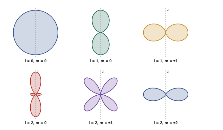
The shapes of \(|Y_l^m|^2\) are the familiar shapes of atomic orbitals, apart from the radial factor. They are symmetric about the \(z\) axis because the \(\phi\) dependence is a pure phase. The dumbbell-shaped \(p_x\) and \(p_y\) orbitals of chemistry are not eigenstates of \(\hat L_z\); they are the real combinations \((Y_1^{-1} \mp Y_1^1)\) up to constants, superpositions of \(m = +1\) and \(m = -1\). Both descriptions are valid bases; chemistry prefers the real ones because they point along bonds.

A numerical check

The program below builds the associated Legendre functions by the standard stable recursions in \(l\), assembles normalized spherical harmonics, and checks orthonormality by integrating over the sphere. It then applies a finite-difference version of the \(\hat L^2\) operator to \(Y_l^m\) and confirms the eigenvalue \(l(l + 1)\).

import cmath, math
def plm(l, m, x):
    """Associated Legendre P_l^m(x) for m >= 0 (no Condon-Shortley sign), by recursion in l."""
    pmm = 1.0
    if m > 0:
        s = math.sqrt((1 - x) * (1 + x)); f = 1.0
        for _ in range(m): pmm *= f * s; f += 2.0
    if l == m: return pmm
    pmp1 = x * (2 * m + 1) * pmm
    if l == m + 1: return pmp1
    for ll in range(m + 2, l + 1):
        pll = ((2 * ll - 1) * x * pmp1 - (ll + m - 1) * pmm) / (ll - m)
        pmm, pmp1 = pmp1, pll
    return pmp1
def Y(l, m, th, ph):
    am = abs(m)
    norm = math.sqrt((2 * l + 1) / (4 * math.pi) * math.factorial(l - am) / math.factorial(l + am))
    eps = (-1) ** m if m > 0 else 1
    return eps * norm * plm(l, am, math.cos(th)) * cmath.exp(1j * m * ph)
print("check: Y_1^0(theta = 0) =", round(Y(1, 0, 0.0, 0.0).real, 6), " sqrt(3/4 pi) =", round(math.sqrt(3 / (4 * math.pi)), 6))
# orthonormality on the sphere: Gauss-like midpoint grid
nt, nph = 120, 60
def inner(l1, m1, l2, m2):
    tot = 0j
    for i in range(nt):
        th = (i + 0.5) * math.pi / nt
        for j in range(nph):
            ph = (j + 0.5) * 2 * math.pi / nph
            tot += Y(l1, m1, th, ph).conjugate() * Y(l2, m2, th, ph) * math.sin(th)
    return tot * (math.pi / nt) * (2 * math.pi / nph)
pairs = [((0, 0), (0, 0)), ((1, 1), (1, 1)), ((2, -1), (2, -1)), ((1, 0), (2, 0)), ((2, 1), (2, -1)), ((3, 2), (1, 0))]
for a, b in pairs:
    v = inner(*a, *b)
    print(f"<Y{a}|Y{b}> = {abs(v):.5f}")
# L^2 / hbar^2 by finite differences on the angular operator, at a sample point
def L2(l, m, th, ph, h=1e-3):
    f = lambda t, p: Y(l, m, t, p)
    d_th = (math.sin(th + h / 2) * (f(th + h, ph) - f(th, ph)) - math.sin(th - h / 2) * (f(th, ph) - f(th - h, ph))) / (h * h * math.sin(th))
    d_ph = (f(th, ph + h) - 2 * f(th, ph) + f(th, ph - h)) / (h * h * math.sin(th) ** 2)
    return -(d_th + d_ph) / f(th, ph)
for l, m in [(1, 0), (1, 1), (2, 1), (3, -2), (4, 3)]:
    print(f"l = {l}, m = {m:2d}:  L^2 / hbar^2 = {L2(l, m, 0.9, 0.4).real:.4f}   l(l+1) = {l * (l + 1)}")
# rigid rotor: CO molecule, E_l = hbar^2 l(l+1) / (2 I)
hbar, u = 1.054571817e-34, 1.66053907e-27
mu = 12.0 * 15.995 / (12.0 + 15.995) * u; r0 = 0.1128e-9
I = mu * r0 ** 2; B = hbar ** 2 / (2 * I)
c = 2.99792458e8; h = 2 * math.pi * hbar
print(f"CO rotational constant B = {B / (h * c) / 100:.4f} per cm; l = 0 -> 1 line at {2 * B / h / 1e9:.1f} GHz")

check: Y_1^0(theta = 0) = 0.488603  sqrt(3/4 pi) = 0.488603
<Y(0, 0)|Y(0, 0)> = 1.00003
<Y(1, 1)|Y(1, 1)> = 1.00000
<Y(2, -1)|Y(2, -1)> = 1.00000
<Y(1, 0)|Y(2, 0)> = 0.00000
<Y(2, 1)|Y(2, -1)> = 0.00000
<Y(3, 2)|Y(1, 0)> = 0.00000
l = 1, m =  0:  L^2 / hbar^2 = 2.0000   l(l+1) = 2
l = 1, m =  1:  L^2 / hbar^2 = 2.0000   l(l+1) = 2
l = 2, m =  1:  L^2 / hbar^2 = 6.0000   l(l+1) = 6
l = 3, m = -2:  L^2 / hbar^2 = 12.0000   l(l+1) = 12
l = 4, m =  3:  L^2 / hbar^2 = 20.0000   l(l+1) = 20
CO rotational constant B = 1.9324 per cm; l = 0 -> 1 line at 115.9 GHz

The finite-difference \(\hat L^2\) returns \(l(l + 1)\) to the printed precision, confirming that the spherical harmonics are its eigenfunctions. The last line applies the eigenvalues to a rotating molecule, a rigid rotor with energy \(\hat L^2/2I\), so \(E_l = \hbar^2l(l + 1)/2I\). Carbon monoxide's lowest rotational transition, near 115 GHz, is the line radio astronomers use to map cold molecular gas, where stars form, across our galaxy and others.

Rotations and conservation

Angular momentum is the generator of rotations, as momentum generates translations: \(e^{-i\alpha\hat L_z/\hbar}\) rotates a wave function by an angle \(\alpha\) about \(z\), as \(e^{-ia\hat p/\hbar}\) shifts it by \(a\). If the Hamiltonian is unchanged by rotations, as for any central potential, it commutes with all three components of \(\hat{\mathbf L}\), so by lesson 9 angular momentum is conserved and \(\hat H\), \(\hat L^2\) and \(\hat L_z\) can be diagonalized together. That is the deep reason the eigenstates of central problems are labeled \(|nlm\rangle\), and why the energy cannot depend on \(m\): all \(2l + 1\) states of a level are related by rotations, which do not change the energy. A magnetic field along \(z\) breaks the symmetry and splits the level into \(2l + 1\) components, the Zeeman effect, discovered by Pieter Zeeman in 1896.