The infinite square well and the superposition principle

The infinite square well, a particle trapped between two impenetrable walls, is the simplest system with discrete energies and the standard first problem of quantum mechanics. PHYS-271 found its energy levels. Here we use it for something more: as a complete worked example of the method of lesson 3. We solve the time-independent equation, prove that the eigenfunctions are orthonormal and complete, expand an arbitrary initial state in them, and follow the state in time. Along the way the well shows the superposition principle at work in its clearest form, including the striking phenomenon of quantum revivals, in which a scrambled wave packet reassembles itself exactly.

Solving the well

Let \(V(x) = 0\) for \(0 < x < a\) and \(V = \infty\) elsewhere. Outside the well the wave function must vanish, since the probability of finding the particle where the potential is infinite is zero. Inside, the time-independent equation is

with general solution \(\psi = A\sin kx + B\cos kx\). The wave function must be continuous, so \(\psi(0) = \psi(a) = 0\). The first condition gives \(B = 0\). The second gives \(A\sin ka = 0\), and since \(A = 0\) would leave no particle, \(ka = n\pi\) with \(n = 1, 2, 3, \ldots\) (negative \(n\) give the same functions with a sign change, and \(n = 0\) gives zero). Normalizing, \(\int_0^a |A|^2\sin^2(n\pi x/a)\,dx = |A|^2a/2 = 1\), so

The slope \(\psi'\) is not continuous at the walls; it jumps from a finite value to zero. That is allowed here because the potential is infinite there, and the usual argument that \(\psi'\) must be continuous (integrate the equation across the point) needs a finite potential. Lesson 6 meets a case where the slope jumps by a definite amount.

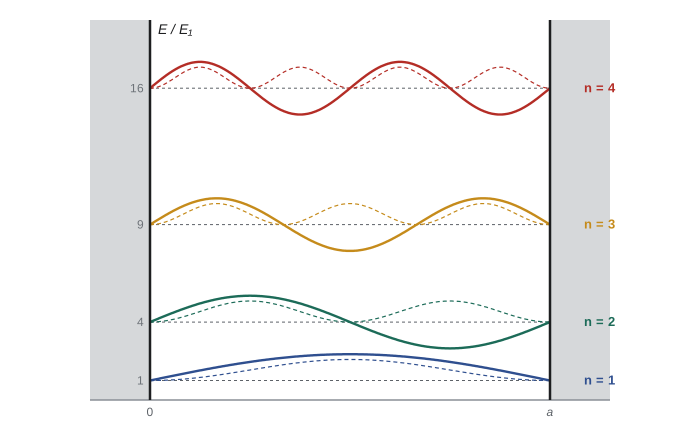
The eigenfunctions display every general property from lesson 3. The energies are real, positive and nondegenerate. The ground state has no nodes, and each higher state adds one. With respect to the middle of the well, the states are alternately even and odd. The spacing \(E_{n+1} - E_n = (2n + 1)E_1\) grows with \(n\), so the levels thin out at high energy, while the fractional spacing \((2n + 1)/n^2\) shrinks, approaching the classical continuum. And the zero-point energy \(E_1 = \pi^2\hbar^2/2ma^2\) is not zero.

Orthonormality

Two different eigenfunctions are orthogonal: for \(m \neq n\),

because each cosine integrates to a sine that vanishes at both ends. Combined with normalization, \(\int\psi_m^{*}\psi_n\,dx = \delta_{mn}\), the Kronecker delta. The eigenfunctions behave like a set of perpendicular unit vectors, with the integral playing the role of the dot product. Lesson 8 shows that this is not special to the box: eigenfunctions of any Hermitian operator with different eigenvalues are orthogonal.

Completeness and expansion

The eigenfunctions are also complete: any function \(f(x)\) on \(0 < x < a\) that is square-integrable can be expanded as \(f = \sum c_n\psi_n\), with the series converging to \(f\) in the sense that the integrated squared error goes to zero. This is Fourier's theorem for sine series, which Joseph Fourier used for heat conduction in 1807 and which Dirichlet put on a rigorous footing in 1829. The coefficients come from orthonormality: multiply \(f = \sum c_n\psi_n\) by \(\psi_m^{*}\), integrate, and every term but one vanishes,

This is Fourier's trick, and it is the same calculation as finding the components of a vector by dotting it with each basis vector. Together, orthonormality and completeness let us treat functions exactly as vectors with infinitely many components, which lesson 8 makes into the formal framework of the theory.

A worked expansion

Suppose a particle starts in the state \(\Psi(x, 0) = Ax(a - x)\), a parabola that vanishes at both walls. Normalizing, \(|A|^2\int_0^a x^2(a - x)^2dx = |A|^2a^5/30 = 1\), so \(A = \sqrt{30/a^5}\). The coefficients are

after two integrations by parts. They vanish for even \(n\), because the parabola is even about the middle of the well and the even-\(n\) eigenfunctions are odd there, and for odd \(n\) they are \(c_n = 8\sqrt{15}/(n\pi)^3\). The ground-state coefficient is \(c_1 = 8\sqrt{15}/\pi^3 = 0.99928\), so \(|c_1|^2 = 0.99856\): the parabola is almost exactly the ground state, and an energy measurement would give \(E_1\) 99.86 times out of 100. The time-dependent state follows at once:

As a check, \(\sum|c_n|^2 = (960/\pi^6)\sum_{n\ \mathrm{odd}} n^{-6} = (960/\pi^6)(\pi^6/960) = 1\), using the known sum of inverse sixth powers over odd integers. The expected energy is \(\langle H\rangle = \sum|c_n|^2E_n\), which can also be computed directly as \(\int\Psi^{*}(-\hbar^2/2m)\Psi''dx = (\hbar^2/2m)(2A^2)\int_0^ax(a - x)\,dx = 5\hbar^2/ma^2\). That is 1.0132 times \(E_1 = 4.935\hbar^2/ma^2\): slightly above the ground-state energy, because of the small admixture of higher states. The program below confirms all of this numerically by projection.

import math
a = 1.0; hbar = m = 1.0
N = 20000; dx = a / N
xs = [(i + 0.5) * dx for i in range(N)]               # midpoint rule
A = math.sqrt(30 / a ** 5)
f = [A * x * (a - x) for x in xs]
psi = lambda n, x: math.sqrt(2 / a) * math.sin(n * math.pi * x / a)
E = lambda n: (n * math.pi * hbar / a) ** 2 / (2 * m)
print(" n   c_n (projection)   c_n (formula)    |c_n|^2")
total, Hsum = 0.0, 0.0
for n in range(1, 40):
    c = sum(psi(n, x) * fx for x, fx in zip(xs, f)) * dx
    exact = 8 * math.sqrt(15) / (n * math.pi) ** 3 if n % 2 else 0.0
    total += c * c; Hsum += c * c * E(n)
    if n <= 7: print(f"{n:2d}   {c: .8f}      {exact: .8f}     {c * c:.6f}")
print(f"sum of |c_n|^2 for n < 40: {total:.8f}")
print(f"<H> from the series: {Hsum:.5f}   direct 5 hbar^2/(m a^2): {5 * hbar ** 2 / (m * a ** 2):.5f}")
print(f"<H> / E1 = {Hsum / E(1):.5f}")
# partial sums of the expansion at the middle of the well
for K in (1, 3, 9):
    s = sum(8 * math.sqrt(15) / (n * math.pi) ** 3 * psi(n, 0.5) for n in range(1, K + 1, 2))
    print(f"partial sum up to n = {K}: Psi(a/2) = {s:.6f}   (true value {A * 0.25:.6f})")

 n   c_n (projection)   c_n (formula)    |c_n|^2
 1    0.99927725       0.99927725     0.998555
 2    0.00000000       0.00000000     0.000000
 3    0.03701027       0.03701027     0.001370
 4    0.00000000       0.00000000     0.000000
 5    0.00799422       0.00799422     0.000064
 6    0.00000000       0.00000000     0.000000
 7    0.00291334       0.00291334     0.000008
sum of |c_n|^2 for n < 40: 1.00000000
<H> from the series: 4.99999   direct 5 hbar^2/(m a^2): 5.00000
<H> / E1 = 1.01321
partial sum up to n = 1: Psi(a/2) = 1.413191   (true value 1.369306)
partial sum up to n = 3: Psi(a/2) = 1.360851   (true value 1.369306)
partial sum up to n = 9: Psi(a/2) = 1.369975   (true value 1.369306)

The partial sums converge rapidly because the coefficients fall as \(1/n^3\), a consequence of the parabola being continuous with a continuous slope inside the well. A wave function with a kink would have coefficients falling only as \(1/n^2\), and one with a jump as \(1/n\), with the slow convergence and overshoot of the Gibbs phenomenon met in PHYS-230.

Sloshing: the two-state superposition

The simplest nonstationary state is a mixture of the two lowest levels, \(\Psi = (\psi_1e^{-iE_1t/\hbar} + \psi_2e^{-iE_2t/\hbar})/\sqrt2\). Its density is

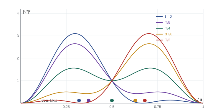
and since \(\psi_1\psi_2\) is positive on the left half of the well and negative on the right, the probability sloshes back and forth with angular frequency \(\omega = (E_2 - E_1)/\hbar = 3\pi^2\hbar/2ma^2\). The expectation value of position is \(\langle x\rangle = a/2 - (16a/9\pi^2)\cos\omega t\), oscillating with amplitude \(0.180a\). This is the quantum version of a particle bouncing between the walls, though with only two components the packet is too broad to look like a particle.

Quantum revivals

Every energy in the well is an integer multiple of \(E_1\), since \(E_n = n^2E_1\). After the revival time \(T_{\mathrm{rev}} = 2\pi\hbar/E_1 = 4ma^2/\pi\hbar\), every phase factor \(e^{-in^2E_1t/\hbar}\) has returned to one, so \(\Psi(x, T_{\mathrm{rev}}) = \Psi(x, 0)\) exactly, whatever the initial state. A narrow wave packet launched in the well spreads, bounces and soon becomes a disordered interference pattern, yet at \(T_{\mathrm{rev}}\) it reassembles perfectly. At simple fractions of \(T_{\mathrm{rev}}\) it re-forms as several smaller copies, a pattern of fractional revivals called the quantum carpet when \(|\Psi|^2\) is plotted against \(x\) and \(t\). Revivals have been observed with wave packets of electrons in highly excited atoms and of molecules vibrating after a short laser pulse. They are a direct test of the superposition principle, since they depend on every component keeping its phase exactly.

Classically, a particle bouncing in the box with energy \(E\) returns to its start after \(2a/v\), which depends on the energy. The quantum revival time does not, because it reflects the integer structure of the spectrum, not the motion of any one component. For an electron in a 1 nm box, \(T_{\mathrm{rev}} = 4m_ea^2/\pi\hbar = 11.0\) fs.

Revivals also make a good test of numerical methods. A program that evolves a wave packet in a box by integrating the Schrödinger equation step by step, as lesson 3 did with Crank–Nicolson, should reproduce the initial state at \(T_{\mathrm{rev}}\). Any loss of the revival reveals errors in the energies of the discretized Hamiltonian, which grow for the high-\(n\) components, so a sharply peaked initial packet, rich in high-\(n\) components, is the hardest case. The same mathematics, phases \(e^{-in^2\theta}\) summed over \(n\), appears in optics as the Talbot effect, in which a grating's image reappears at regular distances behind it, discovered by Henry Fox Talbot in 1836.

The well as a model

Real confining potentials have finite walls (lesson 7), but the infinite well is a good model whenever the walls are much higher than the energies of interest. The electrons in a long conjugated molecule such as beta-carotene move along a chain of alternating single and double bonds, and their absorption wavelengths follow the box formula with \(a\) set by the chain length, which is why longer molecules absorb redder light. Quantum dots, semiconductor crystals a few nanometers across, confine electrons in three dimensions; their emission shifts to the blue as they shrink, roughly as \(1/a^2\), and the 2023 Nobel Prize in Chemistry went to Moungi Bawendi, Louis Brus and Alexei Ekimov for discovering and synthesizing them. Quantum wells in semiconductor lasers, thin layers of one material between layers of another, are one-dimensional boxes engineered to emit at chosen wavelengths.