The wave function and the Born rule

Lesson 1 described a spin, a system with only two possible outcomes, by a two-component vector of amplitudes. A particle moving along a line can be found anywhere, so its state needs an amplitude for every position: a complex-valued function \(\Psi(x, t)\), the wave function. This lesson sets out what the wave function means, how to normalize it, how to compute averages of position and momentum from it, and why the probability it describes is conserved as time passes. These are the working tools for every later lesson. The Schrödinger equation that governs \(\Psi\), met in PHYS-271, is taken here as given; lesson 3 examines it closely.

The statistical interpretation

Max Born proposed in 1926 that the wave function is a probability amplitude for position. Precisely,

The quantity \(|\Psi|^2 = \Psi^{*}\Psi\) is a probability density, with units of inverse length in one dimension. It is not the particle smeared out: a measurement of position always finds the whole particle at one place. Repeat the experiment on many identically prepared particles, and the histogram of results traces out \(|\Psi|^2\). Born received the Nobel Prize in 1954 for this interpretation, which Schrödinger himself never fully accepted; he had hoped the wave described a real distribution of charge.

Because the particle must be somewhere, the total probability must be one:

A wave function that satisfies this is normalized. The Schrödinger equation is linear, so if \(\Psi\) is a solution, so is \(A\Psi\) for any constant \(A\). We use that freedom to normalize: find \(\int|\Psi|^2dx\) and divide \(\Psi\) by its square root. This is possible only for square-integrable functions, ones whose integral of \(|\Psi|^2\) is finite. Functions that blow up, or fail to fall off at infinity, cannot represent physical states. The plane waves of lesson 6 are the important exception, idealizations that are not normalizable on their own but can be superposed into normalizable packets.

Multiplying a normalized wave function by a pure phase \(e^{i\alpha}\) changes nothing measurable, since \(|e^{i\alpha}\Psi|^2 = |\Psi|^2\) and, as we will see, every expectation value is unchanged too. Only relative phases between parts of a superposition have physical consequences, as lesson 1's interference showed.

Probability is conserved

Normalization would be useless if it did not last. Suppose \(\Psi\) is normalized at \(t = 0\). Does it stay normalized as it evolves by the Schrödinger equation

with a real potential \(V\)? Differentiate the total probability under the integral sign:

The Schrödinger equation gives \(\partial_t\Psi = (i\hbar/2m)\,\partial_x^2\Psi - (i/\hbar)V\Psi\), and its complex conjugate gives \(\partial_t\Psi^{*} = -(i\hbar/2m)\,\partial_x^2\Psi^{*} + (i/\hbar)V\Psi^{*}\), using the fact that \(V\) is real. Substituting, the potential terms cancel and

The last step is checked by differentiating the bracket: the cross terms \(\partial_x\Psi^{*}\,\partial_x\Psi\) cancel. The integrand is therefore a total derivative, and its integral is the bracket evaluated at \(\pm\infty\). A normalizable wave function vanishes there, so the total probability does not change. Defining the probability current

we have shown the local continuity equation \(\partial_t|\Psi|^2 + \partial_x j = 0\). Probability, like electric charge, cannot appear or vanish at a point; it can only flow. For a plane wave \(Ae^{ikx}\) the current is \(|A|^2\hbar k/m\), density times velocity \(p/m\), as one would hope. Lessons 6 and 7 use the current to define reflection and transmission probabilities. The proof needed \(V\) to be real; a complex potential, sometimes used to model absorption, makes probability leak away.

Expectation values

If we measure the position of many particles all in the state \(\Psi\), the average of the results is the expectation value

and the average of any function of position is \(\langle f(x)\rangle = \int f(x)|\Psi|^2dx\). The spread of the results is measured by the standard deviation \(\sigma_x\), with \(\sigma_x^2 = \langle x^2\rangle - \langle x\rangle^2\). The expectation value is an average over an ensemble of identical systems, not the result of repeated measurements on one particle, because the first measurement changes the state.

Momentum is subtler, because the wave function is written in terms of position. Consider how \(\langle x\rangle\) changes in time. Differentiating and using the Schrödinger equation as above, then integrating by parts once to remove one derivative,

where the last step integrates by parts once more to combine the two terms of \(j\). It is natural to call \(m\,d\langle x\rangle/dt\) the expectation value of momentum, and the result has the same form as \(\langle x\rangle\) with \(x\) replaced by an operator:

In general, the expectation value of any observable \(Q(x, p)\) is \(\langle Q\rangle = \int \Psi^{*}\,\hat Q\,\Psi\,dx\), with \(\hat Q\) obtained by replacing \(p\) with \(-i\hbar\,\partial_x\). The kinetic energy operator is \(\hat p^2/2m = -(\hbar^2/2m)\partial_x^2\), which is exactly the first term of the Schrödinger equation. The operator is sandwiched between \(\Psi^{*}\) and \(\Psi\); the order matters, since the derivative acts only on the \(\Psi\) to its right.

Why should a derivative represent momentum? A plane wave \(e^{ikx}\) has de Broglie momentum \(\hbar k\), and \(-i\hbar\,\partial_x e^{ikx} = \hbar k\,e^{ikx}\): the momentum operator returns the momentum when it acts on a state of definite momentum. A wave function that wiggles rapidly has large momentum; one that changes slowly has small momentum. For a real wave function, such as a standing wave in a box, \(\langle p\rangle = 0\) because \(\int\psi\psi'dx = [\psi^2/2] = 0\): it contains equal amounts of motion left and right.

Ehrenfest's theorem

Differentiating \(\langle p\rangle\) in the same way gives, after two integrations by parts,

This is Ehrenfest's theorem, published by Paul Ehrenfest in 1927: expectation values obey a form of Newton's second law, with the average force. If the wave packet is narrow compared with the distance over which the force varies, \(\langle -\partial_xV\rangle \approx -V'(\langle x\rangle)\), and the peak of the packet moves like a classical particle. That is how classical mechanics emerges for large objects. For a harmonic oscillator, where the force is linear in \(x\), the relation is exact for any state: \(\langle x\rangle\) oscillates at the classical frequency, as lesson 5 will show.

A Gaussian wave packet

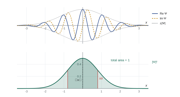
The most useful normalizable state is the Gaussian packet

Its density \(|\Psi|^2\) is a normal distribution with mean \(x_0\) and standard deviation \(\sigma\); the factor \((2\pi\sigma^2)^{-1/4}\) normalizes it. The phase \(e^{ik_0x}\) gives it mean momentum \(\hbar k_0\), and the momentum spread is \(\sigma_p = \hbar/2\sigma\). The product \(\sigma_x\sigma_p = \hbar/2\) is the smallest allowed by the uncertainty principle, which lesson 9 proves. The program below checks these statements by numerical quadrature: it normalizes a packet on a grid, then computes \(\langle x\rangle\), \(\sigma_x\), \(\langle p\rangle\) using a finite-difference derivative, and \(\sigma_p\) from \(\langle p^2\rangle = \hbar^2\int|\partial_x\Psi|^2dx\), which follows from one integration by parts.

import cmath, math
hbar = 1.0                         # natural units: hbar = 1, lengths in nm
x0, sig, k0 = 0.5, 0.8, 6.0         # mean position, width, mean wave number
N, a, b = 4000, -10.0, 11.0
dx = (b - a) / N
xs = [a + i * dx for i in range(N + 1)]
psi = [cmath.exp(-(x - x0) ** 2 / (4 * sig ** 2) + 1j * k0 * x) for x in xs]   # unnormalized
norm = sum(abs(p) ** 2 for p in psi) * dx
psi = [p / math.sqrt(norm) for p in psi]
dens = [abs(p) ** 2 for p in psi]
print(f"norm before {norm:.5f}, after {sum(dens) * dx:.6f}  (exact before: sqrt(2 pi) sigma = {math.sqrt(2 * math.pi) * sig:.5f})")
mean_x = sum(x * d for x, d in zip(xs, dens)) * dx
var_x = sum((x - mean_x) ** 2 * d for x, d in zip(xs, dens)) * dx
dpsi = [(-psi[i + 2] + 8 * psi[i + 1] - 8 * psi[i - 1] + psi[i - 2]) / (12 * dx) for i in range(2, N - 1)]
mean_p = sum(psi[i].conjugate() * (-1j * hbar) * dpsi[i - 2] for i in range(2, N - 1)) * dx
mean_p2 = sum(abs(d) ** 2 for d in dpsi) * dx * hbar ** 2
sx, sp = math.sqrt(var_x), math.sqrt(mean_p2 - mean_p.real ** 2)
print(f"<x> = {mean_x:.4f} (x0 = {x0}),  sigma_x = {sx:.4f} (sigma = {sig})")
print(f"<p> = {mean_p.real:.4f}, imaginary part {abs(mean_p.imag):.1e}  (hbar k0 = {hbar * k0})")
print(f"sigma_p = {sp:.4f}  (hbar / 2 sigma = {hbar / (2 * sig):.4f})")
print(f"sigma_x * sigma_p = {sx * sp:.4f} hbar  (minimum 0.5)")
P_in = sum(d for x, d in zip(xs, dens) if abs(x - x0) <= sig) * dx
print(f"probability within one sigma of x0: {P_in:.4f}  (normal law 0.6827)")

norm before 2.00530, after 1.000000  (exact before: sqrt(2 pi) sigma = 2.00530)
<x> = 0.5000 (x0 = 0.5),  sigma_x = 0.8000 (sigma = 0.8)
<p> = 6.0000, imaginary part 1.2e-16  (hbar k0 = 6.0)
sigma_p = 0.6250  (hbar / 2 sigma = 0.6250)
sigma_x * sigma_p = 0.5000 hbar  (minimum 0.5)
probability within one sigma of x0: 0.6831  (normal law 0.6827)

The imaginary part of \(\langle p\rangle\) comes out at rounding level, as it must: the expectation value of an observable is always real, a property lesson 8 traces to the Hermitian nature of the operators. The small difference between the computed \(\sigma_p\) and \(\hbar/2\sigma\) is far smaller than the printed digits, because the program uses a fourth-order finite-difference derivative; a cruder two-point derivative would make \(\sigma_p\) come out slightly low, even below the bound, a reminder that numerical errors can mimic impossible physics.

Momentum probabilities

The momentum operator gives averages, but the full probability distribution of momentum needs the Fourier transform, which lesson 6 develops: \(\Phi(p) = (2\pi\hbar)^{-1/2}\int\psi(x)e^{-ipx/\hbar}dx\), and \(|\Phi(p)|^2\) is the probability density for momentum, normalized whenever \(\psi\) is. For the Gaussian packet, \(|\Phi|^2\) is again a Gaussian, with mean \(\hbar k_0\) and standard deviation \(\hbar/2\sigma\), which is where the momentum spread quoted above comes from. A wave function that is narrow in position therefore has a broad momentum distribution and the reverse, a reciprocity built into the Fourier transform itself. Position and momentum are two complete descriptions of the same state, and lesson 8 shows that they are simply the components of one state vector in two different bases.

Units and scales

It helps to have numbers in mind. An electron confined to an atom, with \(\sigma_x \approx 0.05\) nm, has \(\sigma_p \geq \hbar/2\sigma_x = 1.1 \times 10^{-24}\) kg m/s and therefore a kinetic energy of order \(\sigma_p^2/2m \approx 4\) eV, the right scale for chemistry. Many quantum calculations become cleaner in units where \(\hbar = m = 1\), as in the code above, and results are converted back at the end. A convenient combination for electrons is \(\hbar^2/2m_e = 0.0381\) eV nm\(^2\), so that a wave number of 1 per nm corresponds to a kinetic energy of 0.0381 eV.