Capstone: the hydrogen atom solved exactly

In January 1926 Schrödinger published the first of his four papers on wave mechanics, and its main result was the energy levels of hydrogen, obtained by solving his new equation for an electron bound to a proton. The Bohr model of 1913, met in PHYS-271, had got the energies right with arbitrary rules and the angular momenta wrong; Schrödinger's equation produced the energies with no extra assumptions, together with the full set of quantum numbers, the degeneracies, the shapes of the orbitals and the probabilities of every measurement. This capstone assembles everything in the course to carry out that calculation completely: separation in spherical coordinates (lesson 10), the spherical harmonics (lesson 11), and a radial equation solved, like the oscillator of lesson 5, by a power series that must terminate. It ends with the spectrum and with the corrections that lie beyond this course.

Setting up the problem

The proton is about 1,836 times heavier than the electron, so to excellent accuracy it stays put and the electron moves in its Coulomb field,

Strictly, the two-body problem reduces to the motion of one particle with the reduced mass \(\mu = m_em_p/(m_e + m_p)\), smaller than \(m_e\) by about one part in 1,800; we use \(m\) for the electron mass and restore \(\mu\) at the end. The potential is central, so lesson 10 applies: \(\psi_{nlm} = R_{nl}(r)Y_l^m(\theta, \phi)\), and \(u = rR\) satisfies

For bound states \(E < 0\). Define \(\kappa = \sqrt{-2mE}/\hbar\), the dimensionless radius \(\rho = \kappa r\) and the constant \(\rho_0 = me^2/(2\pi\epsilon_0\hbar^2\kappa)\). The equation becomes

Limiting forms and the series

At large \(\rho\) the bracket tends to one, so \(u'' \approx u\) and the normalizable solution is \(u \approx e^{-\rho}\). Near the origin the centrifugal term dominates, \(u'' \approx l(l + 1)u/\rho^2\), with solutions \(\rho^{l+1}\) and \(\rho^{-l}\); only the first keeps \(u(0) = 0\). Peel off both limits by writing

Substituting gives \(\rho v'' + 2(l + 1 - \rho)v' + [\rho_0 - 2(l + 1)]v = 0\). Try a power series \(v = \sum_j c_j\rho^j\). Matching coefficients of \(\rho^j\):

The argument from here is the same as for the oscillator. For large \(j\) the recursion becomes \(c_{j+1} \approx 2c_j/j\), the series of \(e^{2\rho}\). If the series never stops, \(v \sim e^{2\rho}\) and \(u \sim \rho^{l+1}e^{\rho}\), which blows up. The series must terminate: for some \(j_{\max}\) the numerator must vanish, \(2(j_{\max} + l + 1) = \rho_0\). Define the principal quantum number \(n = j_{\max} + l + 1\). Then \(\rho_0 = 2n\), and since \(n\) is at least \(l + 1\), the allowed values are \(n = 1, 2, 3, \ldots\) with \(l = 0, 1, \ldots, n - 1\).

The energies

Quantization of \(\rho_0\) is quantization of energy. From \(\rho_0 = 2n\), \(\kappa = me^2/(4\pi\epsilon_0\hbar^2n)\), and \(E = -\hbar^2\kappa^2/2m\):

These are the Bohr energies, now derived. The natural length is the Bohr radius,

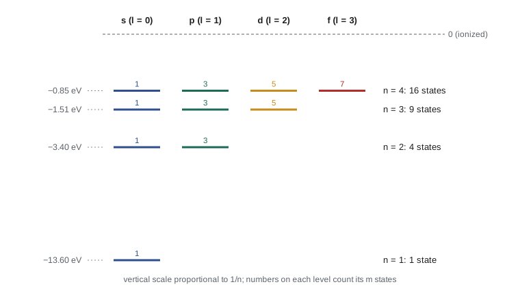
The energy depends only on \(n\). For each \(n\) there are \(n\) values of \(l\), and for each \(l\) there are \(2l + 1\) values of \(m\), so the degeneracy of level \(n\) is \(\sum_{l=0}^{n-1}(2l + 1) = n^2\), and \(2n^2\) once the electron's two spin states are included. The \(m\) degeneracy is required by rotational symmetry, lesson 11. The \(l\) degeneracy is not; it is special to the \(1/r\) potential, the same "accident" that makes classical Kepler orbits close. Wolfgang Pauli explained it in 1926, months before Schrödinger's papers came out in full, by solving hydrogen with matrix mechanics and a hidden conserved quantity, the quantum version of the Runge–Lenz vector, which reveals a larger four-dimensional rotation symmetry. Any departure from a pure \(1/r\) potential, such as the screening by inner electrons in other atoms, lifts the \(l\) degeneracy, which is why the \(2s\) and \(2p\) levels of lithium differ and why subshells fill in the order the periodic table shows.

The wave functions

The terminating series are associated Laguerre polynomials, and the normalized radial functions are

The first few are simple enough to write out:

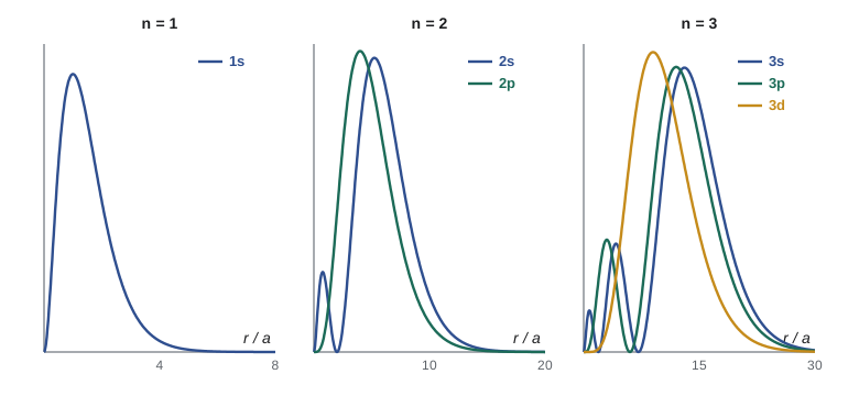
The ground state is \(\psi_{100} = e^{-r/a}/\sqrt{\pi a^3}\), spherically symmetric, with its greatest density at the nucleus but its most probable radius, the peak of \(r^2|R|^2\), exactly at \(r = a\). That is the Bohr radius reinterpreted: not the radius of an orbit, but the most likely distance. The average distance is larger, \(\langle r\rangle = 3a/2\), because of the long exponential tail. In general \(\langle r\rangle = \tfrac{a}{2}[3n^2 - l(l + 1)]\), and the expectation value of the potential energy is \(\langle V\rangle = 2E_n\), so the kinetic energy is \(-E_n\), the quantum form of the virial theorem for a \(1/r\) force. The radial function \(R_{nl}\) has \(n - l - 1\) nodes. States with \(l = n - 1\), the largest allowed, have none and are concentrated near a single radius \(n^2a\), the closest quantum analog of a circular Bohr orbit.

Solving the radial equation numerically

The series solution can be checked by integrating the radial equation directly. The program below uses the Numerov method, a fourth-order scheme for equations of the form \(u'' = f(r)u\), to integrate outward from the origin with \(u \propto r^{l+1}\). For a trial energy, the solution diverges at large \(r\) one way or the other; bisecting on the sign of the divergence finds the energies at which it decays. This is the shooting method of PHYS-271, here applied with the centrifugal term for several values of \(l\). It confirms that the energies are \(-13.6/n^2\) eV whatever \(l\) is, the degeneracy that the series predicts, and it checks the normalization and \(\langle r\rangle\) of the numerical eigenfunctions against the exact formula.

import math
# atomic units: hbar = m = e^2/(4 pi eps0) = 1, so lengths are in Bohr radii and E_n = -1/(2 n^2) hartree
HARTREE_EV = 27.211386
def shoot(E, l, rmax, N=6000):
    h = rmax / N
    f = lambda r: 2 * (-1 / r - E) + l * (l + 1) / r ** 2     # u'' = f(r) u
    r1, r2 = h, 2 * h
    start = lambda r: r ** (l + 1) * (1 - r / (l + 1))     # series near the origin
    u = [0.0, start(r1), start(r2)]
    fs = [0.0, f(r1), f(r2)]
    for i in range(2, N):
        r = (i + 1) * h
        fn = f(r)
        un = (2 * u[i] * (1 + 5 * h * h * fs[i] / 12) - u[i - 1] * (1 - h * h * fs[i - 1] / 12)) / (1 - h * h * fn / 12)
        u.append(un); fs.append(fn)
        if abs(un) > 1e30: break                              # clearly diverging
    return u, h
def tail_sign(E, l, rmax): return math.copysign(1, shoot(E, l, rmax)[0][-1])
def energy(n, l):
    rmax = 8 * n * n + 20
    exact = -0.5 / n ** 2
    lo, hi = exact * 1.08, exact * 0.92                   # bracket around the expected level
    s_lo = tail_sign(lo, l, rmax)
    for _ in range(60):
        mid = 0.5 * (lo + hi)
        if tail_sign(mid, l, rmax) == s_lo: lo = mid
        else: hi = mid
    return 0.5 * (lo + hi), rmax
print(" n  l    E (eV) numerical   -13.6057/n^2    <r> numerical   <r> exact (a/2)(3n^2 - l(l+1))")
for n, l in [(1, 0), (2, 0), (2, 1), (3, 0), (3, 1), (3, 2), (4, 3)]:
    E, rmax = energy(n, l)
    u, h = shoot(E, l, rmax)
    # cut the divergent tail where |u| starts rising again beyond the outermost lobe
    k = len(u) - 1
    while k > 10 and abs(u[k]) > abs(u[k - 1]): k -= 1
    u = u[:k]
    norm = sum(x * x for x in u) * h
    r_mean = sum((i * h) * u[i] ** 2 for i in range(len(u))) * h / norm
    print(f" {n}  {l}    {E * HARTREE_EV:10.5f}       {-HARTREE_EV / (2 * n * n):10.5f}       {r_mean:7.3f}          {0.5 * (3 * n * n - l * (l + 1)):6.3f}")
# Balmer lines from the Bohr energies, with the reduced-mass correction
R_inf = 10973731.568                                      # Rydberg constant, per m
mu_ratio = 1 / (1 + 1 / 1836.15267)
for n2, name in [(3, 'H-alpha'), (4, 'H-beta'), (5, 'H-gamma')]:
    inv = R_inf * mu_ratio * (1 / 4 - 1 / n2 ** 2)
    print(f"{name}: n = {n2} -> 2, vacuum wavelength {1e9 / inv:.2f} nm")

 n  l    E (eV) numerical   -13.6057/n^2    <r> numerical   <r> exact (a/2)(3n^2 - l(l+1))
 1  0     -13.60571        -13.60569         1.500           1.500
 2  0      -3.40143         -3.40142         6.000           6.000
 2  1      -3.40142         -3.40142         5.000           5.000
 3  0      -1.51176         -1.51174        13.500          13.500
 3  1      -1.51174         -1.51174        12.500          12.500
 3  2      -1.51174         -1.51174        10.500          10.500
 4  3      -0.85036         -0.85036        18.000          18.000
H-alpha: n = 3 -> 2, vacuum wavelength 656.47 nm
H-beta: n = 4 -> 2, vacuum wavelength 486.27 nm
H-gamma: n = 5 -> 2, vacuum wavelength 434.17 nm

The numerical energies match \(-13.6057/n^2\) eV to five or six figures, and states with the same \(n\) and different \(l\) come out degenerate, as the series solution predicts. The mean radii agree with \(\tfrac{a}{2}[3n^2 - l(l + 1)]\). The Balmer wavelengths, including the small shift from the reduced mass, are the red, blue-green and violet lines that Johann Balmer fitted with his empirical formula in 1885: H-alpha at 656.5 nm in vacuum, or 656.3 nm in air.

The spectrum

When an electron drops from level \(n_i\) to level \(n_f\), the atom emits a photon of energy \(E_{n_i} - E_{n_f}\), so

the Rydberg formula, with the constant now expressed in fundamental terms. Transitions to \(n_f = 1\) form the ultraviolet Lyman series, to \(n_f = 2\) the visible Balmer series and to \(n_f = 3\) the infrared Paschen series. Not every pair of states is connected: the photon carries one unit of angular momentum and has odd parity, so electric dipole transitions require \(\Delta l = \pm1\) and \(\Delta m = 0, \pm1\), the selection rules that follow from the properties of the spherical harmonics in lesson 11. The reduced mass makes the Rydberg constant slightly different for different isotopes. In 1931 Harold Urey found faint lines displaced from the Balmer lines by about 0.18 nm in concentrated hydrogen, and identified them as coming from deuterium, whose reduced mass is closer to \(m_e\); he received the 1934 Nobel Prize in Chemistry for the discovery.

Beyond this course

Schrödinger's hydrogen atom is not the end of the story. Careful spectroscopy shows that each level splits slightly. The fine structure, about \(10^{-4}\) of the level energies, comes from relativistic corrections to the kinetic energy and from the spin–orbit interaction between the electron's spin and its orbital motion; Dirac's relativistic equation of 1928 accounts for it. The Lamb shift, discovered by Willis Lamb and Robert Retherford in 1947, separates the \(2s_{1/2}\) and \(2p_{1/2}\) levels, which Dirac's theory makes degenerate, by about 1,058 MHz; quantum electrodynamics explains it as the effect of the electromagnetic field's zero-point fluctuations, the vacuum fluctuations of lesson 5. The hyperfine structure, from the interaction with the proton's magnetic moment, splits the ground state by 1,420 MHz, the 21 cm line that radio astronomers use to map hydrogen gas throughout the universe. Today the \(1s\)–\(2s\) transition of hydrogen is measured to about one part in \(10^{15}\), and comparisons of such measurements with theory have tested quantum electrodynamics and pinned down the size of the proton. PHYS-373 continues with spin, perturbation theory and the fine structure; these are the tools that turn the exact solution of this lesson into the precision physics of real atoms.

Looking back over the course, the hydrogen calculation used every idea it developed. The state is a vector, here labeled \(|nlm\rangle\). The observables \(\hat H\), \(\hat L^2\) and \(\hat L_z\) are Hermitian and commute, so their eigenvalues label a complete set of states. Energy quantization comes from normalizability, as in the well and the oscillator. The probability of every measurement is the square of an amplitude. And a superposition of two levels oscillates at the frequency of the light the atom emits. The same structure, with different operators, describes every quantum system studied since 1926.