The free particle, wave packets and the delta-function potential

A particle with no force on it at all should be the easiest problem in quantum mechanics. It turns out to be subtle. The free particle has no normalizable stationary states, so its physical states must be built as wave packets, superpositions of plane waves weighted by a momentum distribution. That construction introduces the Fourier transform and the momentum-space wave function, explains why a packet moves at the classical velocity while its component waves do not, and shows that every packet spreads as it travels. The second half of the lesson takes the simplest potential that can both bind and scatter a particle, the Dirac delta function, and solves it completely. Between them, these problems introduce the distinction between bound states and scattering states that runs through the rest of the course.

Plane waves

With \(V = 0\), the time-independent equation is \(\psi'' = -k^2\psi\) with \(k = \sqrt{2mE}/\hbar\), and its solutions are \(e^{\pm ikx}\). Attaching the time factor gives

a wave moving right for \(k > 0\) and left for \(k < 0\), with momentum \(\hbar k\) and energy \(\hbar^2k^2/2m\). There is no boundary to quantize \(k\): every real wave number, and so every positive energy, is allowed. The spectrum is continuous.

Two things are wrong with plane waves as physical states. First, \(|\Psi_k|^2 = |A|^2\) is the same everywhere, so \(\int|\Psi_k|^2dx\) is infinite and the state cannot be normalized. A particle with exactly known momentum is equally likely to be anywhere in the universe, the extreme case of the uncertainty principle. Second, the wave crests move at the phase velocity \(\omega/k = \hbar k/2m\), which is half the classical velocity \(v = p/m = \hbar k/m\). Both problems disappear when we superpose plane waves into a packet.

Wave packets and the Fourier transform

A normalizable free-particle state is a continuous superposition of plane waves:

This is the free-particle version of lesson 3's expansion \(\sum c_n\psi_ne^{-iE_nt/\hbar}\), with the sum over \(n\) replaced by an integral over \(k\). At \(t = 0\), \(\Psi(x, 0)\) is the inverse Fourier transform of \(\phi(k)\), so Plancherel's theorem gives the coefficient function directly from the initial state:

The theorem also says \(\int|\phi(k)|^2dk = \int|\Psi(x, 0)|^2dx\), so if \(\Psi\) is normalized, \(|\phi(k)|^2\) is a probability density in \(k\). The function \(\Phi(p, t) = \hbar^{-1/2}\phi(p/\hbar)e^{-ip^2t/2m\hbar}\) is the momentum-space wave function, and \(|\Phi(p, t)|^2dp\) is the probability of finding the momentum between \(p\) and \(p + dp\). Position space and momentum space are two descriptions of the same state, related by the Fourier transform, and a state that is narrow in one is broad in the other. For the free particle, \(|\Phi|^2\) does not change in time: with no force, the momentum distribution is conserved, as Ehrenfest's theorem requires.

Group velocity

Suppose \(\phi(k)\) is sharply peaked at \(k_0\). Expand the frequency \(\omega(k) = \hbar k^2/2m\) about \(k_0\): \(\omega \approx \omega_0 + \omega'(k_0)(k - k_0)\). Substituting into the packet,

The integral is a function of \(x - \omega't\) alone: an envelope moving rigidly at the group velocity \(v_g = d\omega/dk = \hbar k_0/m\), which is the classical velocity. The fast carrier wave inside it moves at the phase velocity, half as fast, so the crests are born at the back of the packet and die at the front. This is the same distinction as for water waves or light in a dispersive medium (PHYS-230). Only the group velocity carries the particle, energy and information.

Spreading

The linear approximation ignores the curvature of \(\omega(k)\). Because \(\omega\) is quadratic in \(k\), different momentum components travel at different speeds, and the packet spreads. For a Gaussian the calculation is exact. Start with

The Fourier integral of a Gaussian is a Gaussian, and the time integral can be done by completing the square. The result is a Gaussian whose peak moves at \(v_g\) and whose width grows:

For times short compared with \(\tau = 2m\sigma_0^2/\hbar\) the width barely changes; for long times it grows linearly, \(\sigma \approx \hbar t/2m\sigma_0 = \sigma_pt/m\), the spread you would expect from particles with a spread of velocities \(\sigma_p/m\). Narrow packets spread fastest, because they contain the widest range of momenta. An electron localized to 0.1 nm has \(\tau = 1.7 \times 10^{-16}\) s and doubles its width in about a third of a femtosecond. A grain of dust of mass \(10^{-15}\) kg localized to 1 micron has \(\tau\) of order \(2 \times 10^{7}\) s, most of a year, which is why everyday objects do not visibly blur.

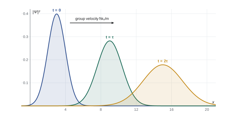
The program below builds the packet by doing the \(k\) integral numerically, as a sum over many plane waves, each advanced in time with its own phase. It then measures the width and mean position and compares them with the exact results.

import cmath, math
hbar = m = 1.0
s0, k0 = 1.0, 3.0                      # initial width and mean wave number
tau = 2 * m * s0 ** 2 / hbar
dk = 0.02
ks = [k0 - 5 + i * dk for i in range(int(10 / dk) + 1)]   # phi is negligible outside k0 +/- 5
phi = [(2 * s0 ** 2 / math.pi) ** 0.25 * math.exp(-s0 ** 2 * (k - k0) ** 2) for k in ks]
print(f"norm in k-space: {sum(p * p for p in phi) * dk:.6f}")
xs = [-12 + 0.1 * i for i in range(561)]  # x from -12 to 44
def packet(t):
    out = []
    for x in xs:
        z = sum(p * cmath.exp(1j * (k * x - hbar * k * k * t / (2 * m))) for p, k in zip(phi, ks))
        out.append(z * dk / math.sqrt(2 * math.pi))
    return out
print("  t/tau   <x>      v_g t    sigma(t)   exact sigma   norm")
for f in (0, 1, 2, 3):
    t = f * tau
    ps = packet(t)
    d = [abs(z) ** 2 for z in ps]
    norm = sum(d) * 0.1
    mx = sum(x * w for x, w in zip(xs, d)) * 0.1 / norm
    sx = math.sqrt(sum((x - mx) ** 2 * w for x, w in zip(xs, d)) * 0.1 / norm)
    exact = s0 * math.sqrt(1 + (hbar * t / (2 * m * s0 ** 2)) ** 2)
    print(f"  {f:4d}   {mx:6.3f}   {hbar * k0 / m * t:6.3f}   {sx:6.4f}     {exact:6.4f}    {norm:.4f}")

norm in k-space: 1.000000
  t/tau   <x>      v_g t    sigma(t)   exact sigma   norm
     0    0.000    0.000   1.0000     1.0000    1.0000
     1    6.000    6.000   1.4142     1.4142    1.0000
     2   12.000   12.000   2.2361     2.2361    1.0000
     3   18.000   18.000   3.1623     3.1623    1.0000

The packet's mean position moves at exactly \(\hbar k_0/m\), and its width grows as the formula predicts, reaching \(\sqrt{10}\,\sigma_0\) at \(t = 3\tau\). The normalization stays at one: the spreading moves probability around but never creates or destroys it.

Bound states and scattering states

The infinite well and the oscillator have only bound states: discrete energies, normalizable eigenfunctions that vanish at infinity, and particles trapped forever. The free particle has only scattering states: a continuum of energies and eigenfunctions that oscillate out to infinity. Most potentials have both. Classically, a particle is bound if its energy is less than the potential at both ends, \(E < V(\pm\infty)\), and free to escape otherwise. In quantum mechanics the same rule applies with tunneling taken into account: if \(V \to 0\) at both ends, states with \(E < 0\) are bound and discrete, and states with \(E > 0\) are scattering states with a continuous spectrum. The rest of this lesson and the next study potentials that have both kinds.

The delta-function well

The Dirac delta function \(\delta(x)\) is an infinitely tall, infinitely narrow spike of unit area: \(\delta(x) = 0\) for \(x \neq 0\) and \(\int f(x)\delta(x)\,dx = f(0)\) for any smooth \(f\). Consider the attractive potential \(V(x) = -\alpha\,\delta(x)\) with \(\alpha > 0\), a model of a very short-range binding force. Away from the origin the particle is free, so for a bound state with \(E < 0\), \(\psi'' = \kappa^2\psi\) with \(\kappa = \sqrt{-2mE}/\hbar\). The normalizable solution is \(\psi = Be^{-\kappa|x|}\), which is already continuous at zero.

The energy comes from the condition on the slope. Integrate the Schrödinger equation from \(-\epsilon\) to \(+\epsilon\):

The delta function makes the slope jump. For \(Be^{-\kappa|x|}\), the slope jumps from \(+\kappa B\) to \(-\kappa B\), a change of \(-2\kappa B\), so \(\kappa = m\alpha/\hbar^2\). Normalizing gives \(B = \sqrt\kappa\). There is exactly one bound state, whatever the strength:

Scattering from the delta function

For \(E > 0\), send a particle in from the left. With \(k = \sqrt{2mE}/\hbar\), the solution is \(Ae^{ikx} + Be^{-ikx}\) for \(x < 0\) (incident plus reflected) and \(Fe^{ikx}\) for \(x > 0\) (transmitted only, since nothing comes in from the right). Continuity at zero gives \(A + B = F\). The slope jump gives \(ik(F - A + B) = -(2m\alpha/\hbar^2)F\). Solving, with \(\beta = m\alpha/\hbar^2k\),

The probability currents of lesson 2 are \(\hbar k|A|^2/m\), \(\hbar k|B|^2/m\) and \(\hbar k|F|^2/m\), so the reflection and transmission probabilities are

with \(R + T = 1\), as conservation of probability demands. Slow particles are mostly reflected, fast ones mostly transmitted, and the crossover is at \(E = m\alpha^2/2\hbar^2\), the magnitude of the bound-state energy. Classically, a particle with any positive energy would pass straight over a well. Quantum particles reflect from it. Strangely, \(R\) and \(T\) depend only on \(\alpha^2\), so a delta-function barrier, \(+\alpha\delta(x)\), scatters exactly as the well does, and a particle at any positive energy tunnels through an infinitely high spike with probability \(T\).

Scattering eigenfunctions are not normalizable, just as for the free particle. They describe steady streams, and \(R\) and \(T\) are ratios of currents. A real experiment sends wave packets, and when the packet is narrow in energy compared with the scale over which \(R\) changes, it splits into a reflected packet with probability \(R\) and a transmitted packet with probability \(T\). The program below computes \(R\) and \(T\) from the matching equations and checks them against the formulas.

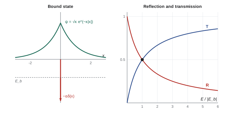
import cmath
hbar = m = 1.0; alpha = 1.0
Eb = -m * alpha ** 2 / (2 * hbar ** 2)
print(f"bound state: kappa = {m * alpha / hbar ** 2:.3f}, E = {Eb:.3f}")
def solve(E, a=alpha):
    k = (2 * m * E) ** 0.5 / hbar
    # unknowns B, F with A = 1: A + B = F and ik(F - A + B) = -(2 m a / hbar^2) F
    # => B - F = -1 and ik B + (ik + 2 m a / hbar^2) F = ik
    g = 2 * m * a / hbar ** 2
    a11, a12, b1 = 1, -1, -1
    a21, a22, b2 = 1j * k, 1j * k + g, 1j * k
    det = a11 * a22 - a12 * a21
    B = (b1 * a22 - a12 * b2) / det
    F = (a11 * b2 - a21 * b1) / det
    return abs(B) ** 2, abs(F) ** 2
print("  E/|Eb|     R        T      R + T   T formula")
for f in (0.1, 0.5, 1.0, 2.0, 10.0):
    E = f * abs(Eb)
    R, T = solve(E)
    Tf = 1 / (1 + m * alpha ** 2 / (2 * hbar ** 2 * E))
    print(f"  {f:5.1f}   {R:.4f}   {T:.4f}   {R + T:.4f}   {Tf:.4f}")
R1, T1 = solve(abs(Eb), a=-alpha)
print(f"barrier (+alpha) at E = |Eb|: R = {R1:.4f}, T = {T1:.4f}  (same as the well)")

bound state: kappa = 1.000, E = -0.500
  E/|Eb|     R        T      R + T   T formula
    0.1   0.9091   0.0909   1.0000   0.0909
    0.5   0.6667   0.3333   1.0000   0.3333
    1.0   0.5000   0.5000   1.0000   0.5000
    2.0   0.3333   0.6667   1.0000   0.6667
   10.0   0.0909   0.9091   1.0000   0.9091
barrier (+alpha) at E = |Eb|: R = 0.5000, T = 0.5000  (same as the well)

The delta function is an idealization, but a useful one: it models any potential much narrower than the wavelength of the particle, such as a thin barrier layer in a semiconductor device or, in three dimensions, the short-range force between a neutron and a nucleus at low energy, where only the integrated strength matters.