Hamiltonian mechanics: Legendre transform and Hamilton's equations

Lagrange's equations are \(n\) second-order equations in the coordinates. In 1834 and 1835 William Rowan Hamilton, then Astronomer Royal of Ireland, recast them as \(2n\) first-order equations in which the coordinates and their conjugate momenta appear on an equal footing. Nothing new is predicted for the motion itself; the gain is in structure. Hamilton's form reveals the geometry of phase space, leads to Liouville's theorem and statistical mechanics, gives the Poisson bracket that became the commutator of quantum mechanics, and suggests numerical methods that respect the physics. This lesson introduces the Hamiltonian through the Legendre transform, derives Hamilton's equations, and shows why integrators built on their structure keep the energy honest over very long times.

Momenta as variables

Lagrangian mechanics uses coordinates and velocities \((q, \dot q)\). Hamilton's idea was to use coordinates and momenta \((q, p)\) instead, with \(p_j = \partial L/\partial\dot q_j\). The momenta are often more natural than the velocities: they are the quantities that are conserved for cyclic coordinates, they appear in Noether charges, and in quantum mechanics they become the operators conjugate to positions. For a particle in Cartesian coordinates, \(p = m\dot x\) and nothing seems to change; but for a charged particle in a magnetic field, \(p = m\dot{\mathbf r} + q\mathbf A\) is not \(m\dot{\mathbf r}\), and for a relativistic particle \(p = \gamma mv\).

The Legendre transform

Replacing one variable by the derivative of a function with respect to it is done with a Legendre transform. Given a convex function \(f(x)\), define \(s = f'(x)\) and

Then \(dg = s\,dx + x\,ds - f'\,dx = x\,ds\), so \(g'(s) = x\): the transform has the old variable as its derivative, and transforming twice returns the original function. Thermodynamics uses the same transform to go from internal energy to enthalpy and free energies, swapping entropy for temperature or volume for pressure. Geometrically, a convex curve can be described either by its points or by its tangent lines, and the Legendre transform switches from one description to the other.

Applied to mechanics, with \(\dot q\) playing the role of \(x\) and \(p\) the role of \(s\), the Hamiltonian is

with every \(\dot q_j\) written in terms of \(q\) and \(p\). This is the energy function \(h\) of lessons 4 and 6, now regarded as a function of momenta instead of velocities. For \(L = \tfrac12 m\dot q^2 - V(q)\), \(p = m\dot q\) and \(H = p^2/2m + V(q)\): kinetic plus potential energy written with momentum. For a pendulum, \(p_\theta = m\ell^2\dot\theta\) and \(H = p_\theta^2/(2m\ell^2) - mg\ell\cos\theta\).

The transform requires that the velocities can be recovered from the momenta, which means the matrix \(\partial^2L/\partial\dot q_j\partial\dot q_k\), the mass matrix, must be invertible. It always is for ordinary mechanical systems. When it is not, as for some systems in field theory, the momenta satisfy constraints of their own and a more elaborate treatment, due to Paul Dirac, is needed.

Hamilton's equations

Take the differential of \(H = \sum p\dot q - L\) in two ways. Directly from the definition,

where the \(d\dot q\) terms cancel because \(p_j = \partial L/\partial\dot q_j\), and Lagrange's equation replaced \(\partial L/\partial q_j\) by \(\dot p_j\). Comparing with \(dH = \sum(\partial H/\partial q_j\,dq_j + \partial H/\partial p_j\,dp_j) + \partial H/\partial t\,dt\) gives Hamilton's equations:

These are \(2n\) first-order equations, and they have a striking symmetry: up to a sign, \(q\) and \(p\) appear in the same way. For \(H = p^2/2m + V\) they read \(\dot q = p/m\) and \(\dot p = -V'(q)\), which together give Newton's law. Along a solution, \(dH/dt = \sum(\partial H/\partial q\,\dot q + \partial H/\partial p\,\dot p) + \partial H/\partial t = \partial H/\partial t\), because the first two terms cancel identically. So \(H\) is conserved whenever it has no explicit time dependence: energy conservation is built into the form of the equations.

Hamilton's equations also follow from a variational principle in phase space. Make the phase-space action \(\int(\sum p\dot q - H)\,dt\) stationary, varying \(q\) and \(p\) independently: varying \(p\) gives \(\dot q = \partial H/\partial p\), and varying \(q\) (with integration by parts) gives \(\dot p = -\partial H/\partial q\). This version of the principle is the one that carries over to quantum mechanics and to the path integral.

Phase space

The \(2n\)-dimensional space of points \((q, p)\) is called phase space. Each point is a complete state of the system, and Hamilton's equations define a velocity field on phase space that moves every state forward. Through each point passes exactly one trajectory, so trajectories never cross. For a system with one degree of freedom and conserved energy, the trajectories are the level curves \(H(q, p) = E\), and the whole phase portrait can be drawn without solving any differential equation.

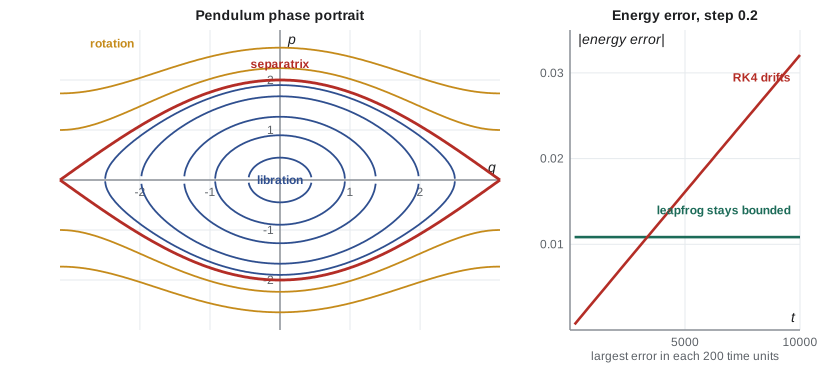
For the pendulum, \(H = p^2/2 - \cos q\) in units with \(m = \ell = g = 1\). Low energies give closed curves around the bottom, librations, where the pendulum swings back and forth. High energies give curves running across all angles, rotations, where the pendulum goes over the top. Between them lies the separatrix at \(H = 1\), passing through the unstable equilibrium at \(q = \pm\pi\), on which the pendulum takes infinitely long to approach the top. Lesson 11 shows that the separatrix is where regular motion first breaks down into chaos when the pendulum is disturbed.

Charged particles

A particle of charge \(q_e\) in an electromagnetic field with scalar potential \(\phi\) and vector potential \(\mathbf A\) has Lagrangian

whose Euler–Lagrange equations give the Lorentz force \(m\ddot{\mathbf r} = q_e(\mathbf E + \dot{\mathbf r}\times\mathbf B)\), with \(\mathbf E = -\nabla\phi - \partial\mathbf A/\partial t\) and \(\mathbf B = \nabla\times\mathbf A\). The canonical momentum is \(\mathbf p = m\dot{\mathbf r} + q_e\mathbf A\), different from the kinetic momentum \(m\dot{\mathbf r}\), and the Hamiltonian is

This minimal-coupling form, replacing \(\mathbf p\) by \(\mathbf p - q_e\mathbf A\), is exactly how the electromagnetic field enters the Schrödinger equation in PHYS-372. The program integrates Hamilton's equations for a particle in a uniform magnetic field and confirms that it returns to its start after one cyclotron period \(2\pi m/q_eB\).

Integrators that respect Hamilton's equations

Hamilton's equations for \(H = T(p) + V(q)\) split naturally into a drift, \(\dot q = \partial T/\partial p\) at fixed \(p\), and a kick, \(\dot p = -\partial V/\partial q\) at fixed \(q\). Each can be solved exactly over a step. The leapfrog or velocity Verlet method, introduced for molecular dynamics by Loup Verlet in 1967, alternates them: half a kick, a full drift, half a kick. Each step is an exact solution of a slightly different Hamiltonian, \(H + O(\Delta t^2)\), so the numerical trajectory exactly conserves a shadow energy close to the true one. The energy error therefore oscillates but does not grow, however long the run. RK4 is more accurate per step but does not have this property, and its energy error drifts steadily.

import math

# 1. The Legendre transform for a relativistic free particle, L = -m c^2 sqrt(1 - v^2/c^2)
m, c = 1.0, 1.0
L = lambda v: -m * c * c * math.sqrt(1 - v * v / (c * c))
for v in (0.1, 0.6, 0.9):
    dv = 1e-6
    p = (L(v + dv) - L(v - dv)) / (2 * dv)                 # p = dL/dv
    H = p * v - L(v)
    print(f"v = {v}c: p = {p:.6f} (gamma m v = {m * v / math.sqrt(1 - v * v):.6f}), "
          f"H = {H:.6f} (sqrt(p^2 c^2 + m^2 c^4) = {math.sqrt(p * p + 1):.6f})")

# 2. Pendulum H = p^2/2 - cos q (units with m = l = g = 1). Compare integrators over many periods.
H = lambda q, p: 0.5 * p * p - math.cos(q)
def leapfrog(q, p, dt):                                  # kick - drift - kick
    p -= 0.5 * dt * math.sin(q); q += dt * p; p -= 0.5 * dt * math.sin(q)
    return q, p
def rk4(q, p, dt):
    f = lambda q, p: (p, -math.sin(q))
    a1, b1 = f(q, p); a2, b2 = f(q + dt / 2 * a1, p + dt / 2 * b1)
    a3, b3 = f(q + dt / 2 * a2, p + dt / 2 * b2); a4, b4 = f(q + dt * a3, p + dt * b3)
    return q + dt / 6 * (a1 + 2 * a2 + 2 * a3 + a4), p + dt / 6 * (b1 + 2 * b2 + 2 * b3 + b4)
q0, p0, dt = 2.0, 0.0, 0.2
E0 = H(q0, p0)
for name, step in (("leapfrog (1 new force per step)", leapfrog), ("RK4 (4 forces per step)        ", rk4)):
    q, p = q0, p0; report = []; worst = 0.0
    for n in range(1, 50001):
        q, p = step(q, p, dt)
        worst = max(worst, abs(H(q, p) - E0))
        if n in (500, 5000, 50000): report.append(f"{worst:.1e}")
    print(f"{name}: largest energy error up to t = 100, 1000, 10000: {', '.join(report)}")

# 3. Hamilton's equations for a charged particle in a uniform field B along z, using p = m v + q A
#    with A = (-B y/2, B x/2, 0): the canonical momentum differs from m v, but the motion is a circle.
qe, B = 1.0, 2.0
def ham_rhs(s):
    x, y, px, py = s
    vx = px + qe * B * y / 2; vy = py - qe * B * x / 2     # dH/dp with m = 1
    return [vx, vy, (qe * B / 2) * vy, -(qe * B / 2) * vx]  # -dH/dq
s = [1.0, 0.0, 0.0, 0.0 + qe * B * 1.0 / 2 + 1.0]          # start at x = 1 moving with v_y = 1
n = 3000; dt = 2 * math.pi / (qe * B) / n
for _ in range(n):                                        # one cyclotron period
    k1 = ham_rhs(s); k2 = ham_rhs([a + dt / 2 * b for a, b in zip(s, k1)])
    k3 = ham_rhs([a + dt / 2 * b for a, b in zip(s, k2)]); k4 = ham_rhs([a + dt * b for a, b in zip(s, k3)])
    s = [a + dt / 6 * (p1 + 2 * p2 + 2 * p3 + p4) for a, p1, p2, p3, p4 in zip(s, k1, k2, k3, k4)]
print(f"after one cyclotron period 2 pi m/(qB) the particle is {math.hypot(s[0] - 1.0, s[1]):.1e} from its start; "
      f"orbit radius m v/(qB) = {1.0 / (qe * B):.2f}")

v = 0.1c: p = 0.100504 (gamma m v = 0.100504), H = 1.005038 (sqrt(p^2 c^2 + m^2 c^4) = 1.005038)
v = 0.6c: p = 0.750000 (gamma m v = 0.750000), H = 1.250000 (sqrt(p^2 c^2 + m^2 c^4) = 1.250000)
v = 0.9c: p = 2.064742 (gamma m v = 2.064742), H = 2.294157 (sqrt(p^2 c^2 + m^2 c^4) = 2.294157)
leapfrog (1 new force per step): largest energy error up to t = 100, 1000, 10000: 1.1e-02, 1.1e-02, 1.1e-02
RK4 (4 forces per step)        : largest energy error up to t = 100, 1000, 10000: 3.3e-04, 3.2e-03, 3.2e-02
after one cyclotron period 2 pi m/(qB) the particle is 5.0e-13 from its start; orbit radius m v/(qB) = 0.50

For the relativistic free particle, \(L = -mc^2\sqrt{1 - v^2/c^2}\), the numerical derivative \(\partial L/\partial v\) reproduces \(\gamma mv\) and the Legendre transform gives \(H = \sqrt{p^2c^2 + m^2c^4}\) to six figures at 0.1, 0.6 and 0.9 times \(c\). For the pendulum released from 2 rad with a large step of 0.2, the leapfrog energy error stays at about \(1.1\times10^{-2}\) whether we run for 100 or 10000 time units, while the RK4 error grows by a factor of ten for every factor of ten in time, from \(3.3\times10^{-4}\) to \(3.2\times10^{-2}\). Over short runs RK4 wins; over long ones the symplectic method wins, even though it uses a quarter of the force evaluations. The charged particle, integrated with canonical momentum and the vector potential \(\mathbf A = (-By/2, Bx/2, 0)\), returns to within \(5\times10^{-13}\) of its start after one cyclotron period.

Why bother with Hamilton?

For solving a given mechanics problem, the Hamiltonian form is rarely quicker than the Lagrangian. Its value lies elsewhere. Statistical mechanics is built on phase space and Liouville's theorem (lesson 10), and its basic quantity, the partition function, is an integral of \(e^{-H/kT}\) over phase space. Quantum mechanics replaces \(q\) and \(p\) by operators whose commutator is \(i\hbar\) times the classical Poisson bracket, and the Hamiltonian becomes the operator in the Schrödinger equation. Perturbation theory for nearly integrable systems, from planetary orbits to particle accelerators, is done with canonical transformations (lesson 11). And long-term numerical simulation of the solar system or of molecules uses symplectic integrators that respect Hamiltonian structure.