Capstone: from classical to modern physics — action, integrability, chaos and the road to quantum mechanics and field theory

This course began with a single number, the action, and a principle that singles out the true motion among all conceivable ones. From it we derived Lagrange's equations, Noether's link between symmetry and conservation, the normal modes of vibrating systems, Hamilton's equations, the geometry of phase space, canonical transformations and the Hamilton–Jacobi equation. This final lesson follows those ideas to the edges of classical mechanics. We ask which systems are solvable, what happens to the others, and how the same structures reappear, almost unchanged, at the foundations of quantum mechanics and field theory.

Integrable systems

A Hamiltonian system with \(n\) degrees of freedom is integrable if it has \(n\) independent conserved quantities \(F_1 = H, F_2, \dots, F_n\) whose Poisson brackets with one another all vanish. The Liouville–Arnold theorem says that for such a system each bounded trajectory lies on an \(n\)-dimensional torus in the \(2n\)-dimensional phase space, and that action-angle variables exist in which \(H = H(J_1, \dots, J_n)\). The motion is then quasi-periodic: each angle advances at its own constant frequency \(\omega_j = \partial H/\partial J_j\). If the frequencies are rationally related, the trajectory closes; if not, it winds around the torus forever, covering it densely.

Almost every system solved in this course and in PHYS-244 is integrable: the harmonic oscillator, the pendulum, the Kepler problem, the symmetric top, any chain of coupled oscillators in the normal-mode approximation. That is no accident: integrable systems are the ones we can solve. But they are exceptional. A generic Hamiltonian with more than one degree of freedom has no conserved quantity besides the energy. The double pendulum, the three-body problem and the asymmetric heavy top are not integrable, and the question of what their motion looks like occupied Poincaré in the 1880s and 1890s and has occupied mathematicians and physicists ever since.

When integrability breaks: the KAM theorem

Suppose we add a small perturbation to an integrable system: a planet's pull on another planet, a slight anharmonicity, a periodic kick. What happens to the invariant tori? Poincaré showed that perturbation series in general diverge, because of small denominators: terms like \(1/(k_1\omega_1 + k_2\omega_2)\) blow up whenever the frequencies are nearly in a rational ratio. It seemed possible that any perturbation, however small, would destroy every torus and make the motion wander over the whole energy surface.

The answer, the Kolmogorov–Arnold–Moser theorem, is more subtle. Andrey Kolmogorov announced it in 1954, Jürgen Moser proved a version for twist maps in 1962, and Vladimir Arnold proved it for Hamiltonian systems in 1963. For a small enough perturbation, most tori survive, slightly deformed: those whose frequency ratios are sufficiently irrational, far from every simple fraction. The tori with rational or nearly rational ratios break up, and in the gaps they leave appear chains of small islands and thin layers of chaotic motion. As the perturbation grows, more tori break, the chaotic layers widen and merge, and eventually chaos spreads over most of phase space.

The standard map

The cleanest place to watch this happen is the standard map, studied by Boris Chirikov in 1979. A rotor, free to turn, receives a sudden kick of strength \(K\) once per period. Its angle \(\theta\) and angular momentum \(p\) just after each kick obey

The map is the exact time evolution over one period of the Hamiltonian \(H = p^2/2 + K\cos\theta\sum_n\delta(t - n)\), so it is area-preserving: its Jacobian matrix \(\begin{pmatrix}1 + K\cos\theta & 1\\ K\cos\theta & 1\end{pmatrix}\) has determinant 1. For \(K = 0\) every orbit has constant \(p\) and lies on a horizontal line, an invariant torus. Plotting the state after each kick for many starting points gives a Poincaré section, the same tool PHYS-244 used for the driven pendulum.

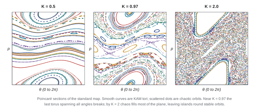
At \(K = 0.5\) most orbits trace smooth curves: KAM tori that survive the kicks. Around the resonance at \(p = 0\) (the pendulum's libration region) lie closed islands, and between them thin chaotic layers along the old separatrices, too thin to see at this scale. The tori that span the whole angle range act as barriers: an orbit below one cannot cross to above it, so \(p\) stays bounded. John Greene showed in 1979 that the last such spanning torus, the one whose rotation number is the golden mean, the most irrational of all numbers, breaks at \(K \approx 0.9716\). Above that value nothing stops an orbit from wandering to arbitrarily large \(p\), and at \(K = 2\) a chaotic sea fills most of the plane, with regular islands around the stable periodic orbits.

import math, random
TWO_PI = 2 * math.pi

# 1. The Chirikov standard map: p' = p + K sin(theta), theta' = theta + p'  (a kicked rotor)
def lyapunov(K, th, p, n=20000):
    # follow a tangent vector with the Jacobian [[1 + K cos th, 1], [K cos th, 1]]
    dth, dp = 1.0, 0.0; s = 0.0
    for _ in range(n):
        c = K * math.cos(th)
        p = p + K * math.sin(th); th = (th + p) % TWO_PI
        dp, dth = dp + c * dth, dth + dp + c * dth
        norm = math.hypot(dth, dp); s += math.log(norm); dth /= norm; dp /= norm
    return s / n
def spread(K, n=2000, orbits=200, seed=1):
    rnd = random.Random(seed); tot = 0.0
    for _ in range(orbits):
        th, p = rnd.uniform(0, TWO_PI), rnd.uniform(-0.1, 0.1); p0 = p
        for _ in range(n):
            p += K * math.sin(th); th = (th + p) % TWO_PI
        tot += (p - p0) ** 2
    return math.sqrt(tot / orbits)
print("   K     Lyapunov exponent (start 0.5, 0.0)   rms change in p after 2000 kicks")
for K in (0.5, 0.9, 1.2, 2.0, 5.0):
    print(f"  {K:3.1f}        {lyapunov(K, 0.5, 0.0):+.4f}                         {spread(K):9.2f}")
print("for K > 4 the momentum diffuses like a random walk: rms about K sqrt(n/2) =", round(5.0 * math.sqrt(2000 / 2), 1))

# 2. How classical is a system? Compare its action with hbar = 1.0546e-34 J s
hbar = 1.0546e-34
cases = [("thrown ball, 0.15 kg, 20 m/s, 2 s", 0.5 * 0.15 * 20 ** 2 * 2.0),
         ("pendulum, 1 kg, 1 m, 5 cm swing, one period", 0.5 * 1.0 * 9.81 * 0.05 ** 2 / 1.0 * 2 * math.pi * math.sqrt(1 / 9.81)),
         ("electron in hydrogen, one orbit (Bohr)", TWO_PI * hbar)]
for name, S in cases:
    print(f"{name:45s} S / hbar = {S / hbar:.1e}")

   K     Lyapunov exponent (start 0.5, 0.0)   rms change in p after 2000 kicks
  0.5        +0.0004                              0.63
  0.9        +0.0002                              0.84
  1.2        +0.2002                              1.53
  2.0        +0.4604                             19.44
  5.0        +0.9436                            166.72
for K > 4 the momentum diffuses like a random walk: rms about K sqrt(n/2) = 158.1
thrown ball, 0.15 kg, 20 m/s, 2 s             S / hbar = 5.7e+35
pendulum, 1 kg, 1 m, 5 cm swing, one period   S / hbar = 2.3e+32
electron in hydrogen, one orbit (Bohr)        S / hbar = 6.3e+00

The program measures the Lyapunov exponent, the average exponential rate at which nearby orbits separate, for an orbit starting at \(\theta = 0.5\), \(p = 0\). For \(K = 0.5\) and 0.9 it is essentially zero (0.0004 and 0.0002, falling toward zero as more kicks are averaged): the orbit is regular. For \(K = 1.2\) it is 0.20, for 2.0 it is 0.46 and for 5.0 it is 0.94: the orbit is chaotic. The spread in momentum after 2000 kicks tells the same story. Below the threshold it stays below 1, because tori trap the orbits. Above it, the spread grows quickly with \(K\), to 1.5 at \(K = 1.2\), where sticky remnants of broken tori still slow the escape, and 19 at \(K = 2\); for \(K = 5\) the spread of 167 is close to the random-walk estimate \(K\sqrt{n/2} = 158\), as if each kick pushed in a random direction. A completely deterministic, area-preserving map has produced behavior indistinguishable from diffusion. That is how chaos underlies the random-looking motion that statistical mechanics assumes.

Chaos in nature

The solar system is a nearly integrable system: each planet would follow a Kepler ellipse if the others were absent. KAM theory explains why it has been stable for billions of years, but it is not the whole story. Jacques Laskar's numerical integrations, beginning in 1989, showed that the inner planets' orbits are chaotic, with a Lyapunov time of about five million years: errors grow by a factor of \(e\) every five million years, so the positions of the planets cannot be predicted beyond about a hundred million years. The gaps in the asteroid belt found by Daniel Kirkwood in 1866, at orbital periods in simple ratios to Jupiter's, are regions where resonances have made orbits chaotic and swept them clear. In particle accelerators, beams circulating billions of times must stay within KAM tori; the dynamic aperture of a storage ring is the region of phase space where that holds.

The road to quantum mechanics

The structures of this course reappear in quantum mechanics with remarkably little change. The old quantum theory of Niels Bohr (1913) and Arnold Sommerfeld (1916) quantized the action variables: \(J = n\hbar\), or more accurately \(J = (n + \tfrac12)\hbar\), so that \(\oint p\,dq = 2\pi\hbar(n + \tfrac12)\). For the oscillator, with \(J = E/\omega_0\), this gives \(E = (n + \tfrac12)\hbar\omega_0\), the exact quantum result. Einstein pointed out in 1917 that this rule makes sense only for integrable systems, whose orbits lie on tori, a remark that was understood only decades later, when the study of quantum chaos began.

Heisenberg's matrix mechanics of 1925 replaced positions and momenta by operators, and Dirac recognized the Poisson bracket structure in it: brackets become commutators over \(i\hbar\), and Hamilton's equations become Heisenberg's. Schrödinger's wave mechanics of 1926 came from the Hamilton–Jacobi equation and the optical analogy of lesson 11: the phase of the wavefunction is \(S/\hbar\). Feynman's path integral of 1948 closed the circle. The quantum amplitude to go from one point to another is a sum over all paths of \(e^{iS/\hbar}\). When \(S\) is enormous compared with \(\hbar\), neighboring paths cancel except near the path where \(S\) is stationary: Hamilton's principle is the classical limit of quantum interference.

How large is \(S/\hbar\) for everyday motion? The program estimates the size of the action, roughly energy times time, for a thrown ball (\(6\times10^{35}\hbar\)) and a gently swinging pendulum (\(2\times10^{32}\hbar\)). For an electron in the lowest Bohr orbit of hydrogen, the action per orbit is \(2\pi\hbar\), about 6 in units of \(\hbar\). Classical mechanics works when \(S/\hbar\) is huge, and fails when it is of order 1. The quantity \(S/\hbar\) is the precise measure of how classical a system is.

The road to field theory

A field, such as the displacement of a vibrating string, the electric potential or the quantum field of an electron, has infinitely many degrees of freedom, one at each point. Lesson 8's chain of masses becomes a string as the spacing shrinks to zero. Its Lagrangian becomes an integral of a Lagrangian density: for a string with mass per length \(\mu\) and tension \(\tau\),

and Hamilton's principle, with the calculus of variations of lesson 2 extended to two variables, gives the wave equation \(\mu\ddot u = \tau u''\). The normal modes of the chain become the standing waves of the string. Electromagnetism has a Lagrangian density, \(\tfrac12\varepsilon_0(E^2 - c^2B^2)\) plus a coupling to charges, from which Maxwell's equations follow. General relativity has the Einstein–Hilbert action, which Hilbert wrote down in 1915, days before Einstein published his field equations. The Standard Model of particle physics is specified by writing down its Lagrangian; its forces come from requiring symmetries of the action, and Noether's theorem gives its conserved charges. The machinery of this course is the language in which the fundamental laws of physics are written.

Looking back

The course started from a practical complaint, that Newton's method becomes clumsy for constrained systems, and found a single principle behind all of mechanics. The calculus of variations gave a general way to turn a stationary integral into a differential equation. Generalized coordinates and Lagrange's equations made constraints disappear, and multipliers brought back their forces when needed. Noether's theorem showed that conservation laws are symmetries. Small oscillations became an eigenvalue problem. Hamilton's form put coordinates and momenta on an equal footing, revealed phase space as an incompressible fluid, and led through canonical transformations to the Hamilton–Jacobi equation and action-angle variables. Integrability turned out to be rare, and its breakdown, governed by the KAM theorem, leads to chaos. And all of it reappears at the foundations of quantum mechanics and field theory, which is why physicists, whatever their field, learn it.