Small oscillations and normal modes: the eigenvalue method

Almost every mechanical system near a stable equilibrium vibrates, and almost every vibration is, to a first approximation, a superposition of independent simple harmonic motions called normal modes. Bridges and buildings sway in them, molecules absorb infrared light at their frequencies, crystals carry sound in them, and the strings and air columns of musical instruments sound at them. PHYS-230 treated two coupled oscillators by hand. This lesson develops the general method: expand the Lagrangian to second order about equilibrium, write it with a mass matrix and a stiffness matrix, and solve a generalized eigenvalue problem. The method handles any number of coordinates at once, and it is how engineers and chemists actually compute vibrations.

Expanding about equilibrium

Consider a system with generalized coordinates \(q_1, \dots, q_n\), a potential \(V(q)\) and a kinetic energy that is a quadratic form in the velocities, \(T = \tfrac12\sum_{jk}m_{jk}(q)\dot q_j\dot q_k\), as it always is for time-independent coordinates. An equilibrium is a point \(q^{(0)}\) where all \(\partial V/\partial q_j = 0\). Let \(\eta_j = q_j - q_j^{(0)}\) be small displacements. Expanding \(V\) to second order (the constant does not matter and the first-order term vanishes at equilibrium) and evaluating the mass coefficients at equilibrium,

Both \(M\) and \(K\) are symmetric matrices, and \(M\) is positive definite because kinetic energy is positive for any motion. The equilibrium is stable if \(K\) is also positive definite, meaning the potential rises in every direction. In matrix form \(L = \tfrac12\dot{\boldsymbol\eta}^{\mathsf T}M\dot{\boldsymbol\eta} - \tfrac12\boldsymbol\eta^{\mathsf T}K\boldsymbol\eta\), and Lagrange's equations are

The eigenvalue problem

Look for solutions in which every coordinate oscillates at the same frequency with fixed relative amplitudes: \(\boldsymbol\eta = \mathbf a\cos(\omega t - \delta)\). Substituting,

This is a generalized eigenvalue problem. The determinant is a polynomial of degree \(n\) in \(\omega^2\), the characteristic equation, whose roots are the squared normal-mode frequencies. For each root the corresponding vector \(\mathbf a\) gives the shape of the mode: the relative amplitude and phase of each coordinate. Because \(M\) and \(K\) are symmetric and \(M\) is positive definite, all \(\omega^2\) are real, and they are positive when \(K\) is positive definite.

The mode shapes are orthogonal with respect to the mass matrix. If \(K\mathbf a_r = \omega_r^2M\mathbf a_r\) and \(K\mathbf a_s = \omega_s^2M\mathbf a_s\), multiplying the first by \(\mathbf a_s^{\mathsf T}\), the second by \(\mathbf a_r^{\mathsf T}\), and subtracting (using symmetry) gives \((\omega_r^2 - \omega_s^2)\,\mathbf a_s^{\mathsf T}M\mathbf a_r = 0\). For distinct frequencies, \(\mathbf a_s^{\mathsf T}M\mathbf a_r = 0\). Normalizing so that \(\mathbf a_r^{\mathsf T}M\mathbf a_r = 1\), define normal coordinates \(\xi_r\) by \(\boldsymbol\eta = \sum_r\xi_r\mathbf a_r\). Then

The Lagrangian has become a sum of independent harmonic oscillators. Any small motion is a superposition of normal modes, each oscillating at its own frequency, with amplitudes and phases set by the initial conditions. The decoupling is exact within the quadratic approximation; nonlinear terms in the full potential couple the modes and let energy pass between them, which is how heat spreads in a solid.

Numerically, the generalized problem is converted to a standard symmetric one. If \(M\) is diagonal, as it is when the coordinates are Cartesian displacements of point masses, write \(\mathbf a = M^{-1/2}\mathbf b\); then \(M^{-1/2}KM^{-1/2}\mathbf b = \omega^2\mathbf b\), a symmetric eigenvalue problem. The program solves it with Jacobi's method of 1846, which zeroes the off-diagonal entries one pair at a time by plane rotations, the same routine PHYS-244 used for the inertia tensor.

The linear triatomic molecule

Carbon dioxide is linear, O=C=O. Model its stretching along the axis as three masses joined by two springs of stiffness \(k\): oxygen masses \(m_O\) at the ends and carbon \(m_C\) in the middle. With displacements \(x_1, x_2, x_3\),

The characteristic equation gives three modes. One has \(\omega = 0\): all three atoms move together, a translation of the molecule with no restoring force. Such zero modes always appear when the potential has a continuous symmetry, a link back to lesson 6. The symmetric stretch, with the carbon at rest and the oxygens moving oppositely, has \(\omega^2 = k/m_O\). The asymmetric stretch, with the oxygens moving together and the carbon moving opposite to them, has \(\omega^2 = (k/m_O)(1 + 2m_O/m_C)\). The ratio of the two frequencies is \(\sqrt{1 + 2m_O/m_C} = 1.915\).

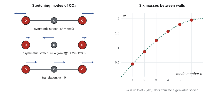
The measured infrared and Raman frequencies of CO\(_2\) are 2349 per centimeter for the asymmetric stretch and 1388 per centimeter for the band usually assigned to the symmetric stretch, a ratio of 1.69 rather than 1.92. The simple model overestimates the ratio for two main reasons: the two C=O bonds interact, so the stiffness matrix has an extra coupling term, and the symmetric stretch mixes with an overtone of the bending vibration (a Fermi resonance), splitting it into a pair of bands near 1285 and 1388 per centimeter. The normal-mode method still applies; it simply needs a more realistic \(K\). The asymmetric stretch near 2349 per centimeter (a wavelength of 4.3 micrometers) and the bending mode near 667 per centimeter (15 micrometers) are the vibrations by which CO\(_2\) absorbs infrared radiation from the Earth's surface.

A chain of masses

Now take \(N\) equal masses \(m\) in a line between two walls, joined by springs of stiffness \(k\). The stiffness matrix is tridiagonal, with \(2k\) on the diagonal and \(-k\) beside it. Try \(a_j = \sin(j\kappa)\): the equation for mass \(j\) becomes \(k(2\sin j\kappa - \sin(j - 1)\kappa - \sin(j + 1)\kappa) = m\omega^2\sin j\kappa\), and the identity \(\sin(j - 1)\kappa + \sin(j + 1)\kappa = 2\cos\kappa\sin j\kappa\) gives \(\omega^2 = (2k/m)(1 - \cos\kappa) = (4k/m)\sin^2(\kappa/2)\). The walls require \(a_0 = a_{N+1} = 0\), so \(\kappa = n\pi/(N + 1)\) with \(n = 1, \dots, N\):

For small \(n\) the frequencies are nearly evenly spaced, like the harmonics of a continuous string; for large \(n\) they bunch up below the maximum \(2\sqrt{k/m}\), because neighboring masses cannot move more oppositely than exactly out of phase. This relation between frequency and wavelength is the dispersion relation of a one-dimensional crystal, and its flattening near the top is the reason sound in solids has a maximum frequency. Peter Debye used exactly this feature in 1912 in his theory of the heat capacity of solids, which PHYS-410 develops.

The triple pendulum

Three equal masses hang in a chain from equal light rods of length \(\ell\). For small angles, the mass matrix in units of \(m\ell^2\) has entries \(M_{jk} = 3 - \max(j, k)\) with \(j, k = 0, 1, 2\), because the top rod's motion carries all three masses, the second carries two, and the third carries one; the stiffness matrix in units of \(mg\ell\) is diagonal, \(\mathrm{diag}(3, 2, 1)\), for the same reason. Now \(M\) is not diagonal, but \(K\) is, so the program uses \(K^{-1/2}\) to symmetrize instead. The three frequencies are 0.645, 1.515 and 2.508 times \(\sqrt{g/\ell}\). In the slowest mode the three rods swing together, nearly like a single pendulum of effective length \(2.4\ell\); in the fastest, neighboring rods swing in opposite directions.

import math

def jacobi(A, tol=1e-12):
    """Eigenvalues and eigenvectors of a real symmetric matrix by Jacobi rotations."""
    n = len(A); A = [row[:] for row in A]; V = [[float(i == j) for j in range(n)] for i in range(n)]
    for _ in range(100):
        off = max(abs(A[i][j]) for i in range(n) for j in range(n) if i != j)
        if off < tol: break
        for p in range(n):
            for q in range(p + 1, n):
                if abs(A[p][q]) < 1e-15: continue
                th = 0.5 * math.atan2(2 * A[p][q], A[q][q] - A[p][p]); c, s = math.cos(th), math.sin(th)
                for k in range(n):
                    akp, akq = A[k][p], A[k][q]; A[k][p], A[k][q] = c * akp - s * akq, s * akp + c * akq
                for k in range(n):
                    apk, aqk = A[p][k], A[q][k]; A[p][k], A[q][k] = c * apk - s * aqk, s * apk + c * aqk
                for k in range(n):
                    vkp, vkq = V[k][p], V[k][q]; V[k][p], V[k][q] = c * vkp - s * vkq, s * vkp + c * vkq
    return [A[i][i] for i in range(n)], V

def modes(M, K):
    """Solve K a = w^2 M a for diagonal M via the symmetric matrix M^-1/2 K M^-1/2."""
    n = len(M); r = [1 / math.sqrt(m) for m in M]
    S = [[r[i] * K[i][j] * r[j] for j in range(n)] for i in range(n)]
    lam, V = jacobi(S)
    out = sorted((max(l, 0.0), [V[i][k] * r[i] for i in range(n)]) for k, l in enumerate(lam))
    return out

# 1. Linear CO2 molecule, stretching along its axis: masses O, C, O joined by two equal springs k
mO, mC = 16.0, 12.0
K = [[1, -1, 0], [-1, 2, -1], [0, -1, 1]]
for w2, a in modes([mO, mC, mO], K):
    big = max(abs(x) for x in a); shape = ", ".join(f"{(round(x / big, 2) or 0.0):+.2f}" for x in a)
    print(f"omega^2 = {w2:.5f} k/u   shape ({shape})")
ratio = math.sqrt(1 + 2 * mO / mC)
print(f"predicted ratio asymmetric/symmetric = sqrt(1 + 2 mO/mC) = {ratio:.3f}; measured 2349/1388 = {2349 / 1388:.3f}")

# 2. Chain of N equal masses between fixed walls: omega_n = 2 sqrt(k/m) sin(n pi / (2(N + 1)))
N = 6
K = [[2.0 if i == j else (-1.0 if abs(i - j) == 1 else 0.0) for j in range(N)] for i in range(N)]
ws = [math.sqrt(w2) for w2, _ in modes([1.0] * N, K)]
print("chain of 6: numerical", " ".join(f"{w:.4f}" for w in ws))
print("            formula  ", " ".join(f"{2 * math.sin(n * math.pi / (2 * (N + 1))):.4f}" for n in range(1, N + 1)))

# 3. Triple pendulum, equal masses and lengths, small swings: M_ij = (3 - max(i, j)) (i, j = 0, 1, 2)
#    in units m l^2, and K = diag(3, 2, 1) m g l. Frequencies in units sqrt(g/l).
M = [[3, 2, 1], [2, 2, 1], [1, 1, 1]]; Kd = [3.0, 2.0, 1.0]
r = [1 / math.sqrt(k) for k in Kd]
# solve M a = (1/w^2) K a  ->  symmetric form K^-1/2 M K^-1/2, eigenvalues 1/w^2
lam, V = jacobi([[r[i] * M[i][j] * r[j] for j in range(3)] for i in range(3)])
print("triple pendulum frequencies (units of sqrt(g/l)):", " ".join(f"{1 / math.sqrt(l):.4f}" for l in sorted(lam, reverse=True)))

omega^2 = 0.00000 k/u   shape (+1.00, +1.00, +1.00)
omega^2 = 0.06250 k/u   shape (-1.00, +0.00, +1.00)
omega^2 = 0.22917 k/u   shape (+0.37, -1.00, +0.37)
predicted ratio asymmetric/symmetric = sqrt(1 + 2 mO/mC) = 1.915; measured 2349/1388 = 1.692
chain of 6: numerical 0.4450 0.8678 1.2470 1.5637 1.8019 1.9499
            formula   0.4450 0.8678 1.2470 1.5637 1.8019 1.9499
triple pendulum frequencies (units of sqrt(g/l)): 0.6448 1.5147 2.5080

The solver finds the CO\(_2\) translation at \(\omega^2 = 0\), the symmetric stretch at \(0.0625\,k/\mathrm u\) (which is \(k/16\), with masses in atomic mass units) with shape \((-1, 0, +1)\), and the asymmetric stretch at \(0.2292\,k/\mathrm u\) with shape \((0.37, -1, 0.37)\). The carbon moves 2.67 times as far as each oxygen, so the center of mass stays put, as it must in a mode with nonzero frequency. The six chain frequencies match the formula to all four printed decimal places.

Instability, zero modes and beats

If \(K\) has a negative eigenvalue, the corresponding \(\omega^2\) is negative and the mode grows exponentially instead of oscillating: the equilibrium is unstable. The bead on the spinning hoop of lesson 4 is an example. Below \(\omega_c\) the single eigenvalue at the bottom is positive; above it, negative. Eigenvalue analysis is how engineers check whether a structure will buckle: as a column's load increases, the lowest stiffness eigenvalue falls and passes through zero at the Euler buckling load.

When two mode frequencies are close, exciting one coordinate excites both modes with similar amplitudes, and the energy sloshes slowly from one coordinate to the other at the difference frequency. PHYS-230 met this as beats between two weakly coupled pendulums. In a building, a tuned mass damper exploits the same physics: a heavy mass on springs near the top, tuned close to the building's lowest mode, draws energy out of the sway and dissipates it.