Constraint forces, Lagrange multipliers and nonholonomic systems

Lesson 4 made a virtue of ignoring constraint forces: by choosing coordinates that satisfy the constraints automatically, the forces that enforce them never appear. Sometimes, though, the constraint force is exactly what we want to know. An engineer needs the tension in a cable, the load on a bearing or the moment a block starts to slide; a physicist needs to know when a particle leaves a surface. And some constraints, such as rolling without slipping on a plane, cannot be built into coordinates at all. This lesson handles both situations with Lagrange multipliers.

Keeping the constraint as an equation

Instead of eliminating a constraint, keep more coordinates than there are degrees of freedom, and impose the constraint \(f(q, t) = 0\) separately. The virtual displacements \(\delta q_j\) are then not independent: they must satisfy \(\sum_j \frac{\partial f}{\partial q_j}\delta q_j = 0\). D'Alembert's principle still says \(\sum_j \big(\frac{d}{dt}\frac{\partial L}{\partial\dot q_j} - \frac{\partial L}{\partial q_j}\big)\delta q_j = 0\) for all such displacements. Adding \(\lambda\) times the constraint condition, with \(\lambda\) chosen to make one bracket vanish, makes all of them vanish:

These \(n\) equations together with \(f = 0\) determine the \(n\) coordinates and \(\lambda(t)\). The right-hand side is the generalized constraint force: \(\lambda\,\partial f/\partial q_j\) is the component of the force that enforces the constraint along \(q_j\). With several constraints \(f_a = 0\), there is one multiplier for each, and the right side becomes \(\sum_a\lambda_a\,\partial f_a/\partial q_j\). The method is the same as the multiplier rule for constrained optimization in MATH-372, now applied in the space of paths.

The geometric meaning is clean. The gradient \(\nabla f\) points perpendicular to the constraint surface \(f = 0\), so the constraint force points perpendicular to it, which is exactly the condition for doing no work in displacements along the surface. The multiplier sets its size.

The pendulum, the other way

Treat a pendulum bob in Cartesian coordinates \((x, y)\) with \(L = \tfrac12 m(\dot x^2 + \dot y^2) - mgy\) and constraint \(f = x^2 + y^2 - \ell^2 = 0\). The equations are

The constraint force is \(2\lambda(x, y)\), along the rod, with magnitude \(2|\lambda|\ell\). To find \(\lambda\), differentiate the constraint twice: \(x\ddot x + y\ddot y + \dot x^2 + \dot y^2 = 0\). Substituting the accelerations gives \(2\lambda\ell^2/m - gy + v^2 = 0\), so \(\lambda = -m(v^2 - gy)/(2\ell^2)\). With \(y = -\ell\cos\theta\) and \(v = \ell\dot\theta\), the tension \(-2\lambda\ell\) is

the familiar result: the rod supports the component of gravity along it and supplies the centripetal force. For a pendulum released from rest at \(\theta_0\), energy gives \(\ell\dot\theta^2 = 2g(\cos\theta - \cos\theta_0)\), so \(T_{\text{rod}} = mg(3\cos\theta - 2\cos\theta_0)\). The program integrates the Cartesian equations with the multiplier and compares.

Leaving a surface

A small bead starts at rest at the top of a smooth hemisphere of radius \(R\), is nudged, and slides down. In polar coordinates \((r, \theta)\) about the center, with \(\theta\) from the top, \(L = \tfrac12 m(\dot r^2 + r^2\dot\theta^2) - mgr\cos\theta\), with constraint \(f = r - R = 0\). The \(r\) equation is

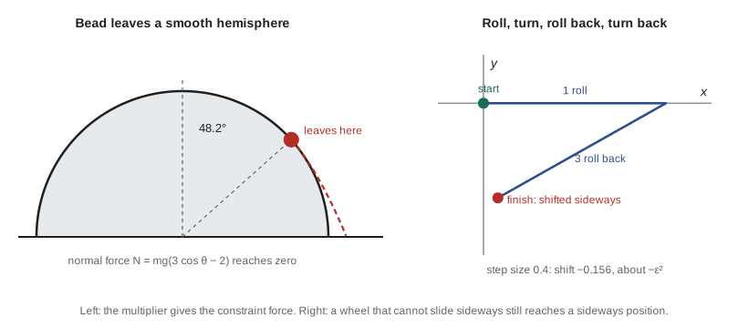
While in contact \(r = R\) and \(\ddot r = 0\), so \(\lambda = mg\cos\theta - mR\dot\theta^2\). This is the radial constraint force, the normal force \(N\) pushing outward. Energy conservation gives \(R\dot\theta^2 = 2g(1 - \cos\theta)\), so \(N = mg(3\cos\theta - 2)\). The surface can only push, not pull, so the bead leaves when \(N\) reaches zero, at \(\cos\theta = 2/3\), or 48.19 degrees from the top, after dropping one third of the radius. The multiplier told us both the force and when the inequality constraint stops acting.

Rolling without slipping

A cylinder of radius \(a\) rolling down an incline of angle \(\alpha\) has two coordinates, the distance \(s\) its center has moved and the angle \(\phi\) it has turned. Rolling without slipping says \(\dot s = a\dot\phi\), which integrates to \(s = a\phi\) plus a constant: the constraint is holonomic, and we can eliminate \(\phi\). With moment of inertia \(I\), \(L = \tfrac12 M\dot s^2 + \tfrac12 I\dot s^2/a^2 + Mgs\sin\alpha\), and \(\ddot s = g\sin\alpha/(1 + I/Ma^2)\): \(\tfrac23 g\sin\alpha\) for a solid cylinder, \(\tfrac12 g\sin\alpha\) for a hoop. Keeping both coordinates and a multiplier instead gives the same acceleration and, in addition, the friction force at the contact, \(\lambda/a = (I/a^2)\ddot s\). That is the force that must be available from static friction; if \(\mu Mg\cos\alpha\) is smaller, the cylinder slips.

Nonholonomic constraints

A wheel rolling on a plane, or a coin, or an ice skate, is different. Take a thin vertical wheel whose contact point is at \((x, y)\) and whose heading is \(\phi\). It can roll forward and it can turn, but it cannot slide sideways, so its velocity must point along its heading:

This is a condition on velocities that cannot be integrated into a relation among \(x\), \(y\) and \(\phi\). Proof: if it could, some function \(g(x, y, \phi) = 0\) would confine the wheel to a two-dimensional surface in its three-dimensional configuration space. But by rolling and turning, the wheel can reach any position with any heading, as anyone who has parallel-parked a car knows. A constraint that restricts velocities without restricting reachable configurations is nonholonomic.

The general form is a constraint linear in velocities, \(\sum_j a_{j}(q)\,\dot q_j = 0\). Nonholonomic constraints cannot be built into coordinates, but they can be handled by multipliers: the equations become \(\frac{d}{dt}\frac{\partial L}{\partial\dot q_j} - \frac{\partial L}{\partial q_j} = \lambda a_{j}\), solved together with the constraint. A caution: one must not substitute a nonholonomic constraint into the Lagrangian before taking derivatives, and the problem cannot be posed as making an action stationary among constrained paths. The correct equations are the d'Alembert form above, which follows the physics of a wheel that grips the ground; making the action stationary among paths that obey the constraint gives a different and physically wrong system, sometimes called vakonomic mechanics.

How a wheel moves sideways

If the wheel cannot slide sideways, how does it ever get sideways? By combining two allowed motions in a loop. Roll forward a distance \(\varepsilon\), turn on the spot by an angle \(\varepsilon\), roll back \(\varepsilon\), turn back \(\varepsilon\). Each step is allowed, but the loop does not close: the wheel ends up displaced sideways by about \(\varepsilon^2\). Mathematically, the two allowed directions of motion, rolling \((\cos\phi, \sin\phi, 0)\) and turning \((0, 0, 1)\), do not commute, and their commutator, called a Lie bracket, is \((\sin\phi, -\cos\phi, 0)\): a sideways motion. The theorem that repeated brackets of allowed motions span every direction, so every configuration is reachable, is due to Wei-Liang Chow in 1939 and Petr Rashevskii in 1938. It underlies the control of robots, cars and spacecraft attitude.

import math
g = 9.81

# 1. Pendulum in Cartesian coordinates with the constraint x^2 + y^2 = l^2 enforced by a multiplier.
#    m xddot = 2 lam x, m yddot = -m g + 2 lam y; differentiating the constraint twice gives lam.
m, l = 0.5, 1.2
def accel(x, y, vx, vy):
    lam = -m * (vx * vx + vy * vy - g * y) / (2 * l * l)   # from x xddot + y yddot + v^2 = 0
    return 2 * lam * x / m, -g + 2 * lam * y / m, lam
th = math.radians(60); x, y = l * math.sin(th), -l * math.cos(th); vx = vy = 0.0
dt = 1e-5; t = 0.0
print(" angle (deg)   tension from multiplier (N)   m(g cos th + l thdot^2) (N)")
for target in (60, 40, 20, 0):
    while math.degrees(math.atan2(x, -y)) > target + 1e-9:
        ax, ay, lam = accel(x, y, vx, vy)
        vx += ax * dt; vy += ay * dt; x += vx * dt; y += vy * dt
        r = math.hypot(x, y); x, y = x * l / r, y * l / r              # project back onto the circle
        vr = (vx * x + vy * y) / l; vx -= vr * x / l; vy -= vr * y / l
    a = math.atan2(x, -y); thdot2 = (vx * vx + vy * vy) / l ** 2
    lam = accel(x, y, vx, vy)[2]
    print(f"   {math.degrees(a):6.2f}        {-2 * lam * l:10.4f}                  {m * (g * math.cos(a) + l * thdot2):10.4f}")
print(f"tension at the bottom from energy: m g (3 - 2 cos 60) = {m * g * (3 - 2 * math.cos(math.radians(60))):.4f} N")

# 2. A bead sliding from rest at the top of a smooth hemisphere: the normal force N = m g (3 cos th - 2)
#    found from the multiplier vanishes at cos th = 2/3.
th_off = math.acos(2 / 3)
print(f"bead leaves the hemisphere at {math.degrees(th_off):.2f} deg from the top, "
      f"having dropped {1 - 2 / 3:.4f} of the radius")

# 3. Nonholonomic constraint: a wheel that cannot slip sideways can still reach any position and heading.
#    Sequence: roll forward, turn on the spot, roll back, turn back. The net result is a sideways shift.
def drive(state, speed, turn_rate, T, n=2000):
    x, y, ph = state; dt = T / n
    for _ in range(n):
        x += speed * math.cos(ph) * dt; y += speed * math.sin(ph) * dt; ph += turn_rate * dt
    return x, y, ph
for eps in (0.4, 0.2, 0.1):
    st = (0.0, 0.0, 0.0)
    for v, w in ((1.0, 0.0), (0.0, 1.0), (-1.0, 0.0), (0.0, -1.0)):
        st = drive(st, v, w, eps)
    print(f"steps of size {eps:.1f}: sideways shift {st[1]:+.5f} m, forward {st[0]:+.5f} m, "
          f"heading {abs(st[2]):.1e} rad, shift / eps^2 = {st[1] / eps ** 2:+.4f}")

 angle (deg)   tension from multiplier (N)   m(g cos th + l thdot^2) (N)
    60.00            2.4525                      2.4525
    40.00            6.3674                      6.3674
    20.00            8.9226                      8.9226
    -0.00            9.8101                      9.8101
tension at the bottom from energy: m g (3 - 2 cos 60) = 9.8100 N
bead leaves the hemisphere at 48.19 deg from the top, having dropped 0.3333 of the radius
steps of size 0.4: sideways shift -0.15577 m, forward +0.03158 m, heading 7.4e-18 rad, shift / eps^2 = -0.9735
steps of size 0.2: sideways shift -0.03973 m, forward +0.00399 m, heading 3.7e-18 rad, shift / eps^2 = -0.9933
steps of size 0.1: sideways shift -0.00998 m, forward +0.00050 m, heading 1.9e-18 rad, shift / eps^2 = -0.9983

The tension from the multiplier and from \(m(g\cos\theta + \ell\dot\theta^2)\) agree at every printed angle, from 2.45 N at the release point to 9.81 N at the bottom, which matches \(mg(3 - 2\cos60^\circ)\) exactly. The bead leaves the hemisphere at 48.19 degrees. For the wheel, steps of 0.4, 0.2 and 0.1 produce sideways shifts of 0.156, 0.040 and 0.010, so the shift divided by \(\varepsilon^2\) approaches 1 as the steps shrink, while the heading returns to its start to rounding error. A car maneuvers into a parking space this way, with steering and driving playing the roles of turning and rolling.