Linear algebra in physics: eigenvalue problems and normal modes

Linear algebra is the hidden engine of computational physics. A circuit of resistors gives a linear system for the node voltages. A finite-difference discretization of a boundary value problem gives a linear system for the grid values. A collection of masses and springs gives an eigenvalue problem whose eigenvalues are the squared frequencies of its normal modes, and a discretized Schrödinger equation gives an eigenvalue problem whose eigenvalues are energy levels. This lesson builds the two central algorithms, Gaussian elimination for linear systems and iterative methods for eigenvalues, and applies them to oscillations of molecules and chains of atoms.

Linear systems and Gaussian elimination

A system \(A\mathbf{x} = \mathbf{b}\) of \(N\) equations in \(N\) unknowns is solved by elimination. For each column in turn, subtract multiples of the pivot row from the rows below to create zeros under the diagonal; then solve the resulting upper triangular system from the bottom up by back substitution. Elimination takes about \(\frac23 N^3\) arithmetic operations and back substitution about \(N^2\). The method appears in the Chinese text The Nine Chapters on the Mathematical Art from around the first century, and is named after Gauss, who used it systematically for least-squares problems in astronomy and geodesy around 1810.

Plain elimination fails if a pivot is zero and is inaccurate if a pivot is small, because dividing by it magnifies rounding errors. Partial pivoting fixes this by swapping rows so that the pivot is the largest available entry in its column. With partial pivoting, Gaussian elimination is backward stable in practice, in the sense of lesson 2: the computed solution is the exact solution of a nearby system. Whether that nearby solution is close to the true one depends on the condition number of the matrix, \(\kappa(A) = \|A\|\,\|A^{-1}\|\), which bounds how much relative errors in \(\mathbf{b}\) or \(A\) can be magnified. With \(\kappa = 10^{k}\), expect to lose about \(k\) of the 16 digits.

Physics often produces matrices with special structure, and exploiting it pays. The tridiagonal matrices of lesson 8 are solved in \(O(N)\) operations by the Thomas algorithm. Symmetric positive definite matrices, such as stiffness matrices of structures and the discrete Laplacian, can be factored as \(A = LL^T\) by Cholesky's method at half the cost of general elimination and with no pivoting. Large sparse systems from three-dimensional grids are solved iteratively, by the relaxation methods of lesson 8 or by the conjugate gradient method of Magnus Hestenes and Eduard Stiefel from 1952.

from fractions import Fraction

def solve(A, b):
    """Gaussian elimination with partial pivoting; A and b are copied."""
    n = len(b)
    M = [row[:] + [b[i]] for i, row in enumerate(A)]
    for k in range(n):
        p = max(range(k, n), key=lambda i: abs(M[i][k]))
        M[k], M[p] = M[p], M[k]
        for i in range(k + 1, n):
            m = M[i][k] / M[k][k]
            for j in range(k, n + 1):
                M[i][j] -= m * M[k][j]
    x = [0] * n
    for i in range(n - 1, -1, -1):
        x[i] = (M[i][n] - sum(M[i][j] * x[j] for j in range(i + 1, n))) / M[i][i]
    return x

# Wheatstone bridge: 10 V source between node 1 and ground; unknown voltages at nodes 1, 2, 3.
# R12 = 100, R13 = 200, R2g = 300, R3g = 400, bridge R23 = 50 ohms, source resistance 1 ohm.
G = lambda r: 1.0 / r
A = [[G(1) + G(100) + G(200), -G(100), -G(200)],
     [-G(100), G(100) + G(300) + G(50), -G(50)],
     [-G(200), -G(50), G(200) + G(400) + G(50)]]
b = [10 * G(1), 0.0, 0.0]
V = solve(A, b)
print("node voltages (V):", " ".join(f"{v:.6f}" for v in V))
print(f"current through the bridge resistor: {(V[1] - V[2]) / 50 * 1000:.4f} mA")

# Ill conditioning: the Hilbert matrix H[i][j] = 1/(i+j+1), with exact solution all ones
print("\n n   max error in float solution   (exact rational arithmetic gives zero error)")
for n in (4, 6, 8, 10, 12):
    H = [[1.0 / (i + j + 1) for j in range(n)] for i in range(n)]
    bh = [sum(row) for row in H]
    x = solve(H, bh)
    Hq = [[Fraction(1, i + j + 1) for j in range(n)] for i in range(n)]
    xq = solve(Hq, [sum(row) for row in Hq])
    print(f"{n:2d}   {max(abs(xi - 1) for xi in x):.2e}                     exact: {all(v == 1 for v in xq)}")

node voltages (V): 9.958240 7.227755 7.067138
current through the bridge resistor: 3.2123 mA

 n   max error in float solution   (exact rational arithmetic gives zero error)
 4   4.56e-13                     exact: True
 6   5.27e-11                     exact: True
 8   1.37e-07                     exact: True
10   7.18e-04                     exact: True
12   5.95e-03                     exact: True

The bridge solution is ordinary and accurate. The Hilbert matrix is the classic ill-conditioned example: its condition number grows roughly like \(e^{3.5N}\), reaching about \(10^{16}\) at \(N = 12\), so the floating-point solution of a system whose exact answer is all ones loses more digits with every increase in \(N\): errors of \(10^{-13}\) at \(N = 4\) grow to nearly \(10^{-2}\) at \(N = 12\), and a few sizes larger the answer has no correct digits at all. The same algorithm in exact rational arithmetic, using Python's Fraction type, returns exactly the right answer, which shows that the trouble is conditioning and rounding, not the algorithm. Hilbert matrices arise in least-squares fitting with the monomials \(1, x, x^2, \ldots\) on \([0, 1]\), which is why lesson 11 fits with better-behaved functions.

Normal modes

Consider masses connected by springs, displaced slightly from equilibrium. Newton's second law for small displacements \(\mathbf{x}\) takes the form

where \(M\) is a diagonal matrix of masses and \(K\) a symmetric stiffness matrix. Looking for solutions in which every mass oscillates at the same frequency, \(\mathbf{x} = \mathbf{v}\cos\omega t\), gives the generalized eigenvalue problem

Each eigenvalue \(\omega^2\) is the square of a normal-mode frequency and each eigenvector \(\mathbf{v}\) the pattern of motion. Because \(K\) and \(M\) are symmetric and \(M\) is positive definite, the eigenvalues are real and the modes are orthogonal with respect to \(M\). Any small motion is a superposition of normal modes, each oscillating independently at its own frequency. Substituting \(\mathbf{v} = M^{-1/2}\mathbf{w}\) converts the problem to the ordinary symmetric eigenvalue problem \(M^{-1/2}KM^{-1/2}\mathbf{w} = \omega^2\mathbf{w}\).

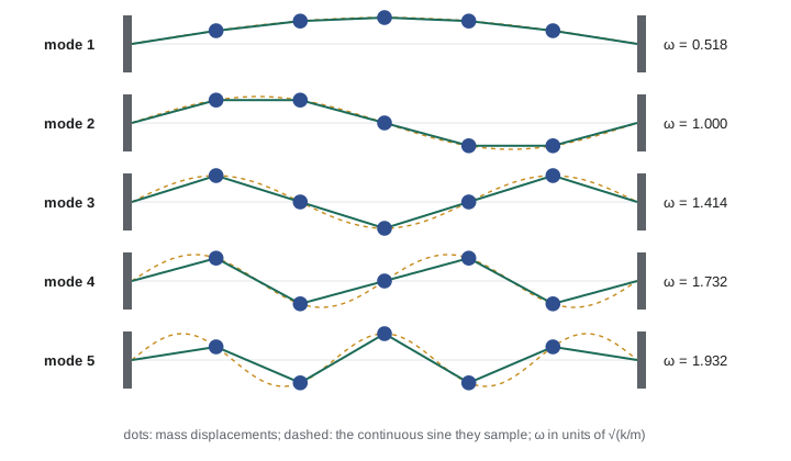
For a chain of \(N\) equal masses \(m\) joined by \(N + 1\) equal springs \(k\) between fixed walls, \(K\) is \(k\) times the tridiagonal matrix with 2 on the diagonal and \(-1\) beside it, the same matrix as the discrete second derivative. Its eigenvalues are known exactly:

For long wavelengths, small \(n\), the frequency is proportional to \(n\), as for a continuous string. For short wavelengths it bends over and reaches a maximum of \(2\sqrt{k/m}\): a discrete chain cannot vibrate faster than this, a fact behind the Debye cutoff of lesson 4 and the phonon spectra of crystals.

Computing eigenvalues

For small matrices the characteristic polynomial \(\det(A - \lambda I)\) can be written down, but its roots are a terrible way to compute eigenvalues: the polynomial's coefficients are extremely sensitive, as James Wilkinson showed with a famous degree-20 example. Practical methods work directly with the matrix.

Power iteration is the simplest. Repeatedly multiply a vector by \(A\) and normalize. Writing the starting vector as a combination of eigenvectors, \(\mathbf{u}_0 = \sum c_i\mathbf{v}_i\), we get \(A^k\mathbf{u}_0 = \sum c_i\lambda_i^k\mathbf{v}_i\), which is dominated by the eigenvector with the largest \(|\lambda|\). The Rayleigh quotient \(\mathbf{u}^T A\mathbf{u}/\mathbf{u}^T\mathbf{u}\) estimates the eigenvalue, with error shrinking like \((\lambda_2/\lambda_1)^{2k}\) for a symmetric matrix. Power iteration with \(A^{-1}\), called inverse iteration, finds the smallest eigenvalue, and with \((A - \sigma I)^{-1}\) the eigenvalue nearest any chosen shift \(\sigma\). Inverse iteration needs a linear solve per step, but it converges quickly when \(\sigma\) is close to an eigenvalue.

To find all eigenvalues of a symmetric matrix, Carl Jacobi's method of 1846 applies a sequence of plane rotations, each chosen to zero one off-diagonal pair. Every rotation reduces the sum of squares of the off-diagonal entries, so the matrix converges to diagonal form; the diagonal holds the eigenvalues and the product of the rotations holds the eigenvectors. Jacobi's method is simple, extremely accurate and easy to program, which suits it to the small matrices of molecular vibrations and coupled oscillators. For large matrices the QR algorithm, discovered independently by John Francis and Vera Kublanovskaya around 1961, is faster and is what libraries use; it was later named one of the top ten algorithms of the twentieth century.

import math

def jacobi_eigen(A, tol=1e-14):
    """All eigenvalues and eigenvectors of a symmetric matrix by Jacobi rotations."""
    n = len(A); A = [row[:] for row in A]
    V = [[float(i == j) for j in range(n)] for i in range(n)]
    for sweep in range(100):
        off = sum(A[i][j]**2 for i in range(n) for j in range(n) if i != j)
        if off < tol: break
        for p in range(n):
            for q in range(p + 1, n):
                if abs(A[p][q]) < 1e-300: continue
                theta = (A[q][q] - A[p][p]) / (2 * A[p][q])
                t = math.copysign(1.0, theta) / (abs(theta) + math.sqrt(theta * theta + 1))
                c = 1 / math.sqrt(t * t + 1); s = t * c
                for k in range(n):                 # rotate columns p and q
                    akp, akq = A[k][p], A[k][q]
                    A[k][p], A[k][q] = c * akp - s * akq, s * akp + c * akq
                for k in range(n):                 # rotate rows p and q
                    apk, aqk = A[p][k], A[q][k]
                    A[p][k], A[q][k] = c * apk - s * aqk, s * apk + c * aqk
                for k in range(n):
                    vkp, vkq = V[k][p], V[k][q]
                    V[k][p], V[k][q] = c * vkp - s * vkq, s * vkp + c * vkq
    vals = [A[i][i] for i in range(n)]
    order = sorted(range(n), key=lambda i: vals[i])
    return [vals[i] for i in order], [[V[k][i] for k in range(n)] for i in order], sweep

def power_iteration(A, iters=200):
    n = len(A); u = [1.0 + 0.1 * i for i in range(n)]
    for _ in range(iters):
        w = [sum(A[i][j] * u[j] for j in range(n)) for i in range(n)]
        norm = math.sqrt(sum(x * x for x in w)); u = [x / norm for x in w]
    Au = [sum(A[i][j] * u[j] for j in range(n)) for i in range(n)]
    return sum(u[i] * Au[i] for i in range(n))

N = 5                                           # chain of five masses, k = m = 1
K = [[2.0 if i == j else (-1.0 if abs(i - j) == 1 else 0.0) for j in range(N)] for i in range(N)]
vals, vecs, sweeps = jacobi_eigen(K)
print(f"chain of {N} masses: Jacobi converged in {sweeps} sweeps")
for n, (lam, v) in enumerate(zip(vals, vecs), start=1):
    exact = 2 * math.sin(n * math.pi / (2 * (N + 1)))
    if v[0] < 0: v = [-x for x in v]
    print(f"  mode {n}: omega = {math.sqrt(lam):.12f}   exact {exact:.12f}   shape " +
          " ".join(f"{x:+.3f}" for x in v))
print(f"power iteration, largest omega^2 = {power_iteration(K):.12f}"
      f" (exact {4 * math.sin(5 * math.pi / 12)**2:.12f})")

# Linear triatomic molecule O=C=O along a line: masses 16, 12, 16; one bond constant k = 1
mO, mC = 16.0, 12.0
Kt = [[1, -1, 0], [-1, 2, -1], [0, -1, 1]]
Mi = [1 / math.sqrt(mO), 1 / math.sqrt(mC), 1 / math.sqrt(mO)]
D = [[Mi[i] * Kt[i][j] * Mi[j] for j in range(3)] for i in range(3)]
vals, vecs, _ = jacobi_eigen(D)
w = [math.sqrt(max(v, 0.0)) for v in vals]
print("\nlinear triatomic O-C-O: omega =", " ".join(f"{x:.5f}" for x in w))
print(f"ratio asymmetric/symmetric stretch = {w[2] / w[1]:.4f};"
      f" formula sqrt(1 + 2 mO/mC) = {math.sqrt(1 + 2 * mO / mC):.4f}")

chain of 5 masses: Jacobi converged in 4 sweeps
  mode 1: omega = 0.517638090205   exact 0.517638090205   shape +0.289 +0.500 +0.577 +0.500 +0.289
  mode 2: omega = 1.000000000000   exact 1.000000000000   shape +0.500 +0.500 +0.000 -0.500 -0.500
  mode 3: omega = 1.414213562373   exact 1.414213562373   shape +0.577 +0.000 -0.577 -0.000 +0.577
  mode 4: omega = 1.732050807569   exact 1.732050807569   shape +0.500 -0.500 +0.000 +0.500 -0.500
  mode 5: omega = 1.931851652578   exact 1.931851652578   shape +0.289 -0.500 +0.577 -0.500 +0.289
power iteration, largest omega^2 = 3.732050807569 (exact 3.732050807569)

linear triatomic O-C-O: omega = 0.00000 0.25000 0.47871
ratio asymmetric/symmetric stretch = 1.9149; formula sqrt(1 + 2 mO/mC) = 1.9149

Jacobi's method reproduces the analytic frequencies to twelve digits in a handful of sweeps, and the eigenvectors are the sampled sine patterns of the figure, normalized. Power iteration also finds the largest eigenvalue to full precision, but it needs a couple of hundred iterations, because the two largest eigenvalues of the chain are close together: the error of the Rayleigh quotient shrinks only by \((\lambda_4/\lambda_5)^2 \approx 0.64\) per iteration.

The triatomic model treats carbon dioxide as three masses on a line joined by two identical springs. It has three eigenvalues: zero, for the uniform translation of the whole molecule, which costs no spring energy; the symmetric stretch, in which the oxygens move outward together while the carbon stays still, at \(\omega_s = \sqrt{k/m_O}\); and the asymmetric stretch, in which the carbon moves against both oxygens, at \(\omega_a = \omega_s\sqrt{1 + 2m_O/m_C}\). The model predicts a frequency ratio of 1.915. The measured infrared and Raman frequencies of carbon dioxide, about 1388 and 2349 per centimeter, give a ratio of 1.69. The difference is modeling error in the sense of lesson 1: real bonds interact, and the symmetric stretch is shifted by a resonance with an overtone of the bending mode, which this one-dimensional model leaves out entirely. The asymmetric stretch is the mode that absorbs infrared radiation near 4.3 micrometers, one of the reasons carbon dioxide is a greenhouse gas.

Eigenvalues of a quantum Hamiltonian

Discretizing the Schrödinger equation \(-\psi'' + V\psi = E\psi\) on a grid with spacing \(h\) and \(\psi = 0\) at both ends turns it into the matrix eigenvalue problem \(H\boldsymbol{\psi} = E\boldsymbol{\psi}\), where \(H\) has \(2/h^2 + V_j\) on the diagonal and \(-1/h^2\) beside it. For the infinite well this is exactly the chain matrix divided by \(h^2\), so its eigenvalues are \(E_n = (4/h^2)\sin^2(n\pi h/2)\), which approach the exact \(n^2\pi^2\) with error \(O(h^2)\) for the low states but are badly wrong for states whose wavelength is comparable with the grid spacing. This is a general lesson: a grid of \(N\) points represents \(N\) states, but only the lower part of its spectrum is physically meaningful. Inverse iteration with a shift near a desired energy, using the Thomas algorithm for each solve, extracts any single level of a large tridiagonal Hamiltonian in \(O(N)\) operations per iteration, a matrix alternative to the shooting of lesson 7.