Capstone: the Ising model from algorithm to phase transition

The capstone brings the course together in one complete computational study: the two-dimensional Ising model of a magnet. It is the simplest system with a genuine phase transition, it has an exact solution against which every number can be checked, and it requires nearly every tool we have built: random numbers and the Metropolis algorithm from lesson 10, careful averages and error bars from lesson 11, verification against exact results in the spirit of lesson 1, and attention to cost and convergence throughout. The goal is not just to produce a graph but to produce one we can defend, with every number accompanied by an honest estimate of its error.

The model

Place a spin \(s_i = \pm 1\) on each site of an \(L \times L\) square lattice. Each spin points up or down, like a tiny bar magnet constrained to two orientations. Neighboring spins prefer to align, and the energy of a configuration is

where the first sum runs over the nearest-neighbor pairs, \(J > 0\) is the coupling and \(h\) an external field, which we set to zero. We use units with \(J = k_B = 1\), so temperature is measured in units of \(J/k_B\). Periodic boundary conditions, in which the right edge wraps round to the left and the top to the bottom, give every spin four neighbors and reduce the effect of the edges. The magnetization per spin \(m = \frac1N\sum s_i\), with \(N = L^2\), measures the order.

At low temperature the energy wins: almost all spins align and \(|m| \approx 1\). At high temperature entropy wins: the spins are nearly random and \(m \approx 0\). In between, at a critical temperature \(T_c\), the system passes through a continuous phase transition, the same kind as the loss of magnetism in iron at its Curie temperature of 1043 K. Wilhelm Lenz proposed the model in 1920 and his student Ernst Ising solved the one-dimensional case in his 1925 thesis, finding no transition at all; he wrongly guessed that none existed in higher dimensions either. Rudolf Peierls gave an argument in 1936 that the two-dimensional model does order at low temperature, and in 1944 Lars Onsager found the exact solution, a landmark of theoretical physics. The critical temperature is

and Chen Ning Yang derived in 1952 the spontaneous magnetization below \(T_c\),

which vanishes at \(T_c\) with the exponent \(\frac18\). These exact results are what make the model such a good test of a simulation.

Step 1: verify on a lattice small enough to solve exactly

A \(4 \times 4\) lattice has \(2^{16} = 65\,536\) configurations, few enough to enumerate. Summing \(e^{-E/T}\) over all of them gives the partition function and exact thermal averages for that lattice, with no statistical error at all. A Metropolis simulation of the same lattice must reproduce them within its error bars. This is verification in its purest form: the small lattice is not physically interesting, but if the simulation code fails here it will fail everywhere, and if it passes, the remaining questions are about statistics and lattice size, not about bugs.

The Metropolis update for the Ising model is especially simple. Flipping spin \(i\) changes the energy by \(\Delta E = 2s_i\sum_{j} s_j\), where the sum is over its four neighbors. The neighbor sum takes only the values \(-4, -2, 0, 2, 4\), so \(\Delta E\) takes only five values and the five acceptance probabilities can be computed once per temperature. One sweep visits every site once, picking sites at random, and is the natural unit of simulation time.

import math, random, itertools

L = 4; N = L * L
nbrs = [[((r + dr) % L) * L + (c + dc) % L for dr, dc in ((0, 1), (1, 0), (0, -1), (-1, 0))]
        for r in range(L) for c in range(L)]
bonds = [(i, nbrs[i][0]) for i in range(N)] + [(i, nbrs[i][1]) for i in range(N)]

hist = {}                                  # count of states for each (E, |M|) pair
for state in itertools.product((-1, 1), repeat=N):
    key = (-sum(state[i] * state[j] for i, j in bonds), abs(sum(state)))
    hist[key] = hist.get(key, 0) + 1
print(f"enumerated {sum(hist.values())} states into {len(hist)} distinct (E, |M|) classes")

def exact(T):
    """Exact averages for the 4x4 periodic lattice from the histogram of all 65 536 states."""
    Z = sE = sE2 = sM = 0.0
    for (E, M), g in hist.items():
        w = g * math.exp(-E / T)
        Z += w; sE += w * E; sE2 += w * E * E; sM += w * M
    e, e2 = sE / Z, sE2 / Z
    return e / N, sM / Z / N, (e2 - e * e) / (T * T * N)

def metropolis(T, sweeps, burn=1000, seed=234):
    rng = random.Random(seed)
    s = [1] * N
    acc = {d: math.exp(-d / T) for d in (4, 8)}
    E = -sum(s[i] * s[j] for i, j in bonds)
    sE = sE2 = sM = 0.0
    for sweep in range(sweeps + burn):
        for _ in range(N):
            i = rng.randrange(N)
            dE = 2 * s[i] * sum(s[j] for j in nbrs[i])
            if dE <= 0 or rng.random() < acc[dE]:
                s[i] = -s[i]; E += dE
        if sweep >= burn:
            sE += E; sE2 += E * E; sM += abs(sum(s))
    e, e2 = sE / sweeps, sE2 / sweeps
    return e / N, sM / sweeps / N, (e2 - e * e) / (T * T * N)

print("4x4 lattice: exact enumeration against Metropolis (40 000 sweeps)")
print("   T     <E>/N exact  Metropolis    <|m|> exact  Metropolis    C exact  Metropolis")
for T in (1.5, 2.27, 3.0):
    ex, mc = exact(T), metropolis(T, 40000)
    print(f"{T:5.2f}   {ex[0]:10.5f}  {mc[0]:10.5f}    {ex[1]:10.5f}  {mc[1]:10.5f}    "
          f"{ex[2]:7.4f}  {mc[2]:8.4f}")

enumerated 65536 states into 45 distinct (E, |M|) classes
4x4 lattice: exact enumeration against Metropolis (40 000 sweeps)
   T     <E>/N exact  Metropolis    <|m|> exact  Metropolis    C exact  Metropolis
 1.50     -1.95064    -1.95043       0.98617     0.98610     0.2003    0.2006
 2.27     -1.56499    -1.56000       0.84360     0.84093     0.7836    0.7929
 3.00     -1.01707    -1.00968       0.60129     0.59819     0.6031    0.6053

The simulation agrees with exact enumeration to two or three decimal places at all three temperatures, including the critical region, where fluctuations are largest. The remaining differences are the size expected from 40 000 correlated sweeps. With this check passed we trust the update rule, the energy bookkeeping and the measurement code.

Step 2: simulate a larger lattice across the transition

Now we move to a lattice large enough to show the transition, \(L = 12\) with 144 spins, small enough that the whole scan runs in a few seconds of Python, and scan temperatures from 1.5 to 3.5. At each temperature the simulation starts from the final configuration of the previous one, which shortens equilibration, discards the first 300 sweeps and then measures for 1500 sweeps. The heat capacity per spin comes from the energy fluctuations, \(C = (\langle E^2\rangle - \langle E\rangle^2)/(T^2N)\), and the susceptibility from the magnetization fluctuations, \(\chi = N(\langle m^2\rangle - \langle |m|\rangle^2)/T\). Using fluctuations avoids numerical differentiation of noisy averages, a trick from statistical mechanics that is also a lesson in numerical analysis.

Step 3: error bars that respect correlations

Successive sweeps of a Markov chain are correlated, especially near \(T_c\), where large clusters of aligned spins form and dissolve slowly. Treating 1500 sweeps as 1500 independent samples would understate the error. The blocking method, analyzed by Henrik Flyvbjerg and Henrik Petersen in 1989, groups the time series into blocks long enough to be nearly independent, averages each block, and computes the standard error from the scatter of the block averages. As the block length grows the estimated error rises and then levels off once blocks are longer than the correlation time; that plateau is the honest error bar. The ratio of the squared blocked error to the naive one estimates \(2\tau_{\text{int}}\), where \(\tau_{\text{int}}\) is the integrated autocorrelation time, the number of sweeps per effectively independent sample.

import math, random

def run(L, temps, sweeps=1500, burn=300, seed=234):
    rng = random.Random(seed); N = L * L
    nb = [[((r + dr) % L) * L + (c + dc) % L for dr, dc in ((0, 1), (1, 0), (0, -1), (-1, 0))]
          for r in range(L) for c in range(L)]
    s = [1] * N
    E = -sum(s[i] * (s[nb[i][0]] + s[nb[i][1]]) for i in range(N))
    results = []
    for T in temps:
        acc = {4: math.exp(-4 / T), 8: math.exp(-8 / T)}
        Es, Ms = [], []
        for sweep in range(sweeps + burn):
            for _ in range(N):
                i = rng.randrange(N)
                dE = 2 * s[i] * (s[nb[i][0]] + s[nb[i][1]] + s[nb[i][2]] + s[nb[i][3]])
                if dE <= 0 or rng.random() < acc[dE]:
                    s[i] = -s[i]; E += dE
            if sweep >= burn:
                Es.append(E / N); Ms.append(abs(sum(s)) / N)
        results.append((T, Es, Ms))
    return results

def blocked_error(x, block):
    nb = len(x) // block
    means = [sum(x[k * block:(k + 1) * block]) / block for k in range(nb)]
    mu = sum(means) / nb
    return math.sqrt(sum((m - mu)**2 for m in means) / (nb - 1) / nb)

def onsager_m(T):
    return (1 - math.sinh(2 / T) ** -4) ** 0.125 if T < 2 / math.log(1 + math.sqrt(2)) else 0.0

L = 12; N = L * L
temps = [1.5, 1.8, 2.0, 2.1, 2.2, 2.3, 2.4, 2.6, 3.0, 3.5]
print(f"L = {L}, 1500 measured sweeps per temperature; Tc = {2 / math.log(1 + math.sqrt(2)):.4f}")
print("   T     <|m|>     error   Onsager |m|    <E>/N      C        chi    tau_int")
for T, Es, Ms in run(L, temps):
    n = len(Es)
    m = sum(Ms) / n; e = sum(Es) / n
    C = N * (sum(x * x for x in Es) / n - e * e) / T**2
    chi = N * (sum(x * x for x in Ms) / n - m * m) / T
    naive = math.sqrt(sum((x - m)**2 for x in Ms) / (n - 1) / n)
    err = blocked_error(Ms, 100)
    tau = 0.5 * (err / naive) ** 2 if naive > 0 else 0.0
    print(f"{T:5.2f}   {m:.4f}   {err:.4f}   {onsager_m(T):10.4f}   {e:8.4f}   {C:6.3f}   {chi:7.2f}   {tau:6.1f}")

L = 12, 1500 measured sweeps per temperature; Tc = 2.2692
   T     <|m|>     error   Onsager |m|    <E>/N      C        chi    tau_int
 1.50   0.9864   0.0007       0.9865    -1.9507    0.201      0.03      1.3
 1.80   0.9612   0.0021       0.9569    -1.8696    0.394      0.09      3.2
 2.00   0.9062   0.0098       0.9113    -1.7378    0.749      0.42     12.2
 2.10   0.8744   0.0128       0.8687    -1.6693    0.889      0.74     11.3
 2.20   0.8112   0.0215       0.7848    -1.5596    1.119      1.53     14.8
 2.30   0.7184   0.0198       0.0000    -1.4188    1.346      2.19      8.4
 2.40   0.5440   0.0481       0.0000    -1.2591    1.337      4.12     25.3
 2.60   0.3761   0.0217       0.0000    -1.0434    0.783      2.68      7.3
 3.00   0.2235   0.0134       0.0000    -0.8231    0.422      1.30      4.9
 3.50   0.1806   0.0097       0.0000    -0.6701    0.267      0.68      4.3

Step 4: interpret the results

The table tells the story of the transition. Well below \(T_c\) the magnetization agrees with Yang's exact formula to within the error bars. As \(T\) rises toward \(T_c\) the simulated \(|m|\) stays above the exact infinite-lattice value, and above \(T_c\) it does not drop to zero but tails off gradually. That is not an error in the simulation but a finite-size effect: a finite lattice cannot have a true phase transition, because its partition function is a finite sum of smooth functions, and on a \(12 \times 12\) lattice a fluctuation that flips a large fraction of the spins is not rare. The heat capacity and susceptibility peak near, but slightly above, 2.269, and on larger lattices their peaks grow taller, narrower and move toward \(T_c\). The way they scale with \(L\), studied systematically by finite-size scaling theory, is how simulations extract critical exponents for models that have no exact solution.

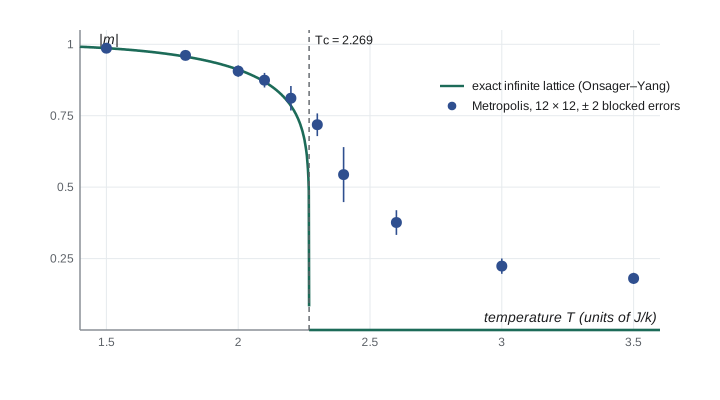
The autocorrelation time column shows critical slowing down: far from \(T_c\) a few sweeps suffice for an independent sample, but near \(T_c\) it takes tens of sweeps, and on larger lattices the growth continues roughly as \(L^z\) with \(z \approx 2\) for single-spin Metropolis updates. Precision near \(T_c\) is therefore expensive. Cluster algorithms cure this by flipping whole clusters of aligned spins at once, chosen so that detailed balance still holds: the Swendsen–Wang algorithm of 1987 and the Wolff algorithm of 1989 reduce critical slowing down dramatically and are the standard tools for studying critical points.

Step 5: what to report

A defensible computational result states the model and its parameters, the algorithm and its settings (lattice size, boundary conditions, sweeps, equilibration, seed), the verification performed, and every number with an error bar computed in a way appropriate to correlated data. It identifies the main systematic effects, here the finite lattice size and the finite run length near \(T_c\), and says how they would be reduced. It makes the code available so that another person can rerun it with the same seed and get the same numbers. These are the same standards that apply to an experiment, and for the same reasons.

Looking back over the course

Every lesson of this course appeared in some form in this capstone. Floating-point care, from lesson 2, kept the energy as an integer sum and avoided accumulating rounding errors over millions of updates. The error analysis of lessons 1 and 3 became the statistical error analysis of lessons 10 and 11. The verification against an exact small case echoed the comparisons with exact pendulum periods, quadrature values and eigenvalues. The cost estimates of lesson 1 decided the lattice size and number of sweeps that fit in a few seconds, and the stability concerns of lessons 5 and 8 reappeared as the correlation and equilibration of a Markov chain. The specific algorithms will change as you move on to larger problems, compiled languages and parallel computers, but the habits carry over unchanged: understand the physics, choose a method whose errors you can estimate, verify it on a case you can solve, measure its convergence, and report what you found with an honest statement of how well you know it.

Natural next steps from here include molecular dynamics of many particles with the Verlet integrator of lesson 6 and neighbor lists, spectral methods for partial differential equations built on the FFT of lesson 11, the time-dependent Schrödinger equation by Crank–Nicolson from lesson 8, and Monte Carlo studies of other lattice models with cluster algorithms. Each builds directly on the tools of this course.