Data analysis: fitting, uncertainty and the fast Fourier transform

Computation in physics is not only about solving equations; it is equally about extracting reliable conclusions from data, whether the data come from a laboratory or from a simulation. Two tools dominate. Least-squares fitting finds the parameters of a model that best describe measurements and, done properly, says how uncertain those parameters are and whether the model fits at all. The Fourier transform decomposes a signal into frequencies, revealing periodicities hidden in noise, and the fast Fourier transform computes it so efficiently that it underlies everything from spectroscopy to the processing of gravitational-wave data. This lesson builds both from scratch.

Uncertainty in a measurement

Repeated measurements \(x_1, \ldots, x_N\) of the same quantity scatter. Their mean \(\bar x\) estimates the true value, the sample standard deviation \(s = \sqrt{\sum(x_i - \bar x)^2/(N - 1)}\) estimates the scatter of a single measurement, and the standard error \(s/\sqrt N\) estimates the uncertainty of the mean. The divisor \(N - 1\) rather than \(N\), Bessel's correction, accounts for the fact that \(\bar x\) was estimated from the same data. A result is reported as \(\bar x \pm s/\sqrt N\), meaning that the true value lies within that range about 68% of the time if the errors are random and roughly Gaussian.

When a result \(q = f(x, y, \ldots)\) is computed from independent measured quantities, small uncertainties propagate as

For products and quotients this means relative uncertainties add in quadrature, and for a power \(q = x^n\) the relative uncertainty is multiplied by \(|n|\). The formula assumes the uncertainties are small enough for a linear approximation and the inputs are uncorrelated. When either assumption fails, a Monte Carlo approach is safer: draw many random inputs from their distributions, compute \(q\) for each, and take the spread of the results.

Fitting a straight line

Suppose we measure \(y_i\) at known \(x_i\), each with uncertainty \(\sigma_i\), and expect \(y = a + bx\). The principle of least squares, published by Adrien-Marie Legendre in 1805 and justified by Gauss in 1809 as the most probable estimate for Gaussian errors, chooses \(a\) and \(b\) to minimize

Setting the partial derivatives to zero gives two linear equations. With weights \(w_i = 1/\sigma_i^2\) and sums \(S = \sum w_i\), \(S_x = \sum w_ix_i\), \(S_y = \sum w_iy_i\), \(S_{xx} = \sum w_ix_i^2\), \(S_{xy} = \sum w_ix_iy_i\), and \(\Delta = SS_{xx} - S_x^2\), the solution is

The parameter uncertainties follow from propagating the \(\sigma_i\) through these formulas. The intercept and slope are usually correlated, with covariance \(-S_x/\Delta\), which matters when both are used together, for instance to predict \(y\) at a new \(x\). Choosing the origin of \(x\) near the weighted mean of the data removes the correlation.

The minimum value of \(\chi^2\) tests the model. If the model is right and the \(\sigma_i\) are honest, \(\chi^2_{\min}\) follows a chi-squared distribution with \(\nu = N - 2\) degrees of freedom, whose mean is \(\nu\). The reduced chi-squared \(\chi^2_{\min}/\nu\) should therefore be near 1. A value much larger than 1 means the model is wrong or the uncertainties are underestimated; a value much smaller means the uncertainties are overestimated. The residuals \(y_i - a - bx_i\) should scatter randomly about zero; a systematic curve in the residuals betrays a missing term in the model even when \(\chi^2\) looks acceptable.

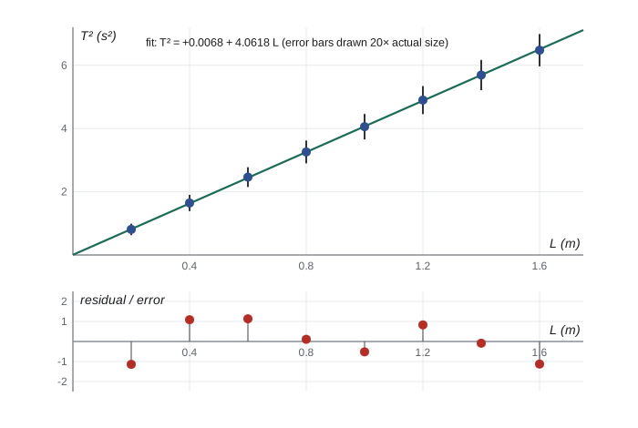
A pendulum experiment illustrates this. For small swings \(T^2 = (4\pi^2/g)L\), so a plot of \(T^2\) against \(L\) should be a straight line through the origin with slope \(4\pi^2/g\). The program generates data as an experiment would, with a fixed random seed: eight lengths from 0.2 to 1.6 m, periods timed with a random error of 0.005 s, and an amplitude of \(15^\circ\), large enough that the finite-amplitude correction of lesson 1 slightly increases every period. It then fits the line and examines the result.

import math, random

rng = random.Random(208)
g_true, amp = 9.81, math.radians(15)
corr = 1 + amp**2 / 16 + 11 * amp**4 / 3072          # finite-amplitude factor from lesson 1
lengths = [0.2 * k for k in range(1, 9)]
sigT = 0.005
data = []
for L in lengths:
    T = 2 * math.pi * math.sqrt(L / g_true) * corr + rng.gauss(0, sigT)
    data.append((L, T * T, 2 * T * sigT))             # y = T^2 with propagated error 2 T sigma_T

def fit_line(pts):
    w = [1 / s**2 for _, _, s in pts]
    S = sum(w); Sx = sum(wi * x for wi, (x, _, _) in zip(w, pts)); Sy = sum(wi * y for wi, (_, y, _) in zip(w, pts))
    Sxx = sum(wi * x * x for wi, (x, _, _) in zip(w, pts)); Sxy = sum(wi * x * y for wi, (x, y, _) in zip(w, pts))
    D = S * Sxx - Sx * Sx
    b = (S * Sxy - Sx * Sy) / D; a = (Sxx * Sy - Sx * Sxy) / D
    chi2 = sum(((y - a - b * x) / s)**2 for x, y, s in pts)
    return a, b, math.sqrt(Sxx / D), math.sqrt(S / D), chi2

a, b, sa, sb, chi2 = fit_line(data)
nu = len(data) - 2
g = 4 * math.pi**2 / b; sg = g * sb / b
print(" L (m)    T^2 (s^2)   error    residual/error")
for x, y, s in data:
    print(f"{x:5.2f}   {y:9.5f}   {s:.5f}   {(y - a - b * x) / s:+6.2f}")
print(f"\nintercept a = {a:+.5f} +- {sa:.5f} s^2   slope b = {b:.5f} +- {sb:.5f} s^2/m")
print(f"chi^2 = {chi2:.2f} for {nu} degrees of freedom (reduced {chi2 / nu:.2f})")
print(f"g from slope = {g:.4f} +- {sg:.4f} m/s^2  (true 9.81)")
print(f"g after dividing out the amplitude correction = {g * corr**2:.4f} +- {sg * corr**2:.4f} m/s^2")

 L (m)    T^2 (s^2)   error    residual/error
 0.20     0.80895   0.00899    -1.14
 0.40     1.64549   0.01283    +1.09
 0.60     2.46166   0.01569    +1.13
 0.80     3.25827   0.01805    +0.11
 1.00     4.05826   0.02015    -0.52
 1.20     4.89932   0.02213    +0.83
 1.40     5.69130   0.02386    -0.09
 1.60     6.47711   0.02545    -1.13

intercept a = +0.00683 +- 0.00929 s^2   slope b = 4.06182 +- 0.01277 s^2/m
chi^2 = 5.99 for 6 degrees of freedom (reduced 1.00)
g from slope = 9.7194 +- 0.0305 m/s^2  (true 9.81)
g after dividing out the amplitude correction = 9.8032 +- 0.0308 m/s^2

The fit is good: the residuals scatter on both sides of zero and the reduced chi-squared is close to 1. Yet the value of \(g\) from the slope is low by almost 1%, three times its statistical uncertainty. The cause is not noise but a systematic error, the finite-amplitude correction, which multiplies every period by the same factor and so cannot be seen in the residuals at all. Only physics knowledge reveals it, and removing it brings \(g\) into agreement with the true value. The lesson is general: a good \(\chi^2\) shows that the data are consistent with the model, not that the model is complete.

Beyond straight lines

Any model that is linear in its parameters, such as a polynomial \(y = \sum c_k x^k\) or a sum of known functions \(y = \sum c_k\phi_k(x)\), leads to a linear system for the parameters, the normal equations \((A^TWA)\mathbf{c} = A^TW\mathbf{y}\), where \(A_{ik} = \phi_k(x_i)\). Forming \(A^TWA\) squares the condition number of the problem, and for monomials on \([0, 1]\) it produces the ill-conditioned Hilbert matrices of lesson 9. Better practice uses orthogonal polynomials or solves the least-squares problem with a QR factorization, which avoids squaring the condition number.

Models that are nonlinear in their parameters, such as \(y = A e^{-t/\tau}\cos(\omega t + \phi)\), need an iterative minimizer. The Gauss–Newton method linearizes the model about the current parameters, solves the resulting linear least-squares problem for a correction, and repeats. Kenneth Levenberg in 1944 and Donald Marquardt in 1963 added a damping term that makes the iteration robust far from the minimum, and the Levenberg–Marquardt method is the standard nonlinear fitter. A tempting shortcut, linearizing the model by a transformation such as taking logarithms of exponential decay data, changes the error distribution and biases the fit unless the weights are transformed too: if \(y\) has uncertainty \(\sigma\), then \(\ln y\) has uncertainty \(\sigma/y\).

When the error distribution is unknown or the model is awkward, the bootstrap of Bradley Efron, from 1979, estimates uncertainties by brute force: resample the data with replacement many times, refit each resampled set, and take the spread of the fitted parameters. It is a Monte Carlo method in the spirit of lesson 10, and it needs nothing but a fitting routine and a random number generator.

The discrete Fourier transform

A signal sampled at \(N\) equally spaced times \(t_n = n\,\Delta t\) can be written as a sum of complex exponentials,

where \(X_k\) is the amplitude at frequency \(f_k = k/(N\Delta t)\). The frequency spacing \(1/(N\Delta t)\) is the reciprocal of the total duration, so a longer record resolves finer frequency differences. The highest frequency that can be represented is the Nyquist frequency \(f_N = 1/(2\Delta t)\), half the sampling rate, a limit identified by Harry Nyquist in 1928 and made precise by Claude Shannon in 1949. A sinusoid above \(f_N\) is not lost but aliased: its samples are identical to those of a lower frequency, and it appears in the spectrum at the wrong place. The cure is to filter out high frequencies before sampling, which is why audio is recorded at 44.1 kHz, a little more than twice the 20 kHz limit of human hearing.

The power spectrum \(|X_k|^2\) shows how the signal's energy is distributed in frequency, and Parseval's theorem \(\sum|x_n|^2 = \frac1N\sum|X_k|^2\) says the total is the same in both descriptions. If a sinusoid does not complete a whole number of cycles in the record, its power spreads into neighboring frequencies, an effect called spectral leakage. Multiplying the data by a smooth window such as the Hann window \(\sin^2(\pi n/N)\), named after Julius von Hann, before transforming suppresses the leakage at the cost of slightly broader peaks.

The fast Fourier transform

Computing the \(N\) sums directly takes about \(N^2\) complex multiplications. In 1965 James Cooley and John Tukey published an algorithm that does it in about \(N\log_2 N\). For \(N = 2^m\), split the sum into even and odd terms:

Each half is a transform of length \(N/2\), and because \(E_k\) and \(O_k\) repeat with period \(N/2\), the two half-length transforms give all \(N\) outputs: \(X_k = E_k + w^kO_k\) and \(X_{k+N/2} = E_k - w^kO_k\) with \(w = e^{-2\pi i/N}\). Applying the split recursively gives \(\log_2 N\) levels of \(N\) operations each. For a million points the saving is a factor of about 50 000. Gauss had found essentially the same algorithm around 1805 while interpolating the orbits of asteroids, but his work, written in Latin and published only after his death, went unnoticed until after Cooley and Tukey's paper. The FFT is widely counted among the most important algorithms ever devised.

import cmath, math, random

def fft(x):
    """Recursive radix-2 Cooley-Tukey FFT; len(x) must be a power of 2."""
    n = len(x)
    if n == 1: return list(x)
    even, odd = fft(x[0::2]), fft(x[1::2])
    out = [0j] * n
    for k in range(n // 2):
        t = cmath.exp(-2j * math.pi * k / n) * odd[k]
        out[k], out[k + n // 2] = even[k] + t, even[k] - t
    return out

def dft(x):
    n = len(x)
    return [sum(x[m] * cmath.exp(-2j * math.pi * k * m / n) for m in range(n)) for k in range(n)]

rng = random.Random(234)
N, dt = 1024, 0.01                               # 10.24 s sampled at 100 Hz; Nyquist 50 Hz
sig = [math.sin(2 * math.pi * 7.0 * n * dt) + 0.5 * math.sin(2 * math.pi * 12.5 * n * dt)
       + 0.3 * math.sin(2 * math.pi * 83.0 * n * dt) + rng.gauss(0, 1.0) for n in range(N)]
small = sig[:64]
print("FFT matches direct DFT on 64 points:", max(abs(a - b) for a, b in zip(fft(small), dft(small))) < 1e-9)
X = fft(sig)
power = [abs(X[k])**2 / N for k in range(N // 2)]
df = 1 / (N * dt)
print(f"frequency resolution {df:.4f} Hz, Nyquist frequency {1 / (2 * dt):.0f} Hz")
floor = sorted(power)[N // 4]                       # median power: a robust noise level
peaks = [k for k in range(1, N // 2 - 1)
         if power[k] > 10 * floor and power[k] >= power[k - 1] and power[k] >= power[k + 1]]
for k in peaks:
    print(f"  peak at {k * df:6.3f} Hz (bin {k}), power {power[k]:7.1f},"
          f" with adjacent bins {power[k - 1] + power[k] + power[k + 1]:7.1f}")
print("the 83 Hz tone is above the Nyquist frequency and appears aliased at 100 - 83 = 17 Hz")
print(f"median noise power per bin {floor:.2f}; expected peak power A^2 N / 4 =",
      ", ".join(f"{A * A * N / 4:.0f}" for A in (1.0, 0.5, 0.3)))
pt = sum(v * v for v in sig); pf = sum(abs(c)**2 for c in X) / N
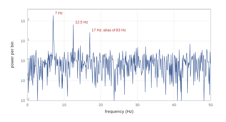
print(f"Parseval check: sum |x|^2 = {pt:.4f}, sum |X|^2 / N = {pf:.4f}")

FFT matches direct DFT on 64 points: True
frequency resolution 0.0977 Hz, Nyquist frequency 50 Hz
  peak at  7.031 Hz (bin 72), power   191.6, with adjacent bins   249.8
  peak at 12.500 Hz (bin 128), power    66.7, with adjacent bins    68.0
  peak at 16.992 Hz (bin 174), power    26.5, with adjacent bins    29.1
the 83 Hz tone is above the Nyquist frequency and appears aliased at 100 - 83 = 17 Hz
median noise power per bin 0.76; expected peak power A^2 N / 4 = 256, 64, 23
Parseval check: sum |x|^2 = 1699.5114, sum |X|^2 / N = 1699.5114

The FFT agrees with the direct sum to rounding error. In the time series the noise is as large as the strongest tone and the signal looks like random scribble, yet the spectrum shows sharp peaks near 7 Hz, at 12.5 Hz and near 17 Hz, standing a hundred times above the median noise level. The 17 Hz peak is the 83 Hz tone aliased: sampled at 100 Hz, a sinusoid at 83 Hz is indistinguishable from one at 17 Hz. The tone at 12.5 Hz falls exactly on bin 128 and its power matches the expected \(A^2N/4 = 64\) to within the noise. The 7 Hz tone falls between bins 71 and 72, so its power leaks into its neighbors: the peak bin holds 192 of the expected 256, and the peak bin and its two neighbors together hold 250. The noise power is spread evenly over all 512 bins, while each tone's power is concentrated in one or two, which is why a long record pulls a weak periodic signal out of strong noise. The same principle lets radio astronomers find pulsars and lets LIGO's matched filters find gravitational-wave chirps.