Why computational physics: models, algorithms and error

Most of the equations of physics cannot be solved with pencil and paper. A pendulum swinging through a large angle, a planet tugged by its neighbors, a guitar string with stiffness, heat flowing through an irregular wall, a magnet made of a million interacting spins: each is described by laws we know well, yet the solutions have no closed form. Computational physics is the craft of getting reliable numbers out of such laws. It sits beside theory and experiment as a third way of doing physics. Theory supplies the equations and the limiting cases, experiment supplies the data and the final verdict, and computation connects the two by turning equations into predictions that can be compared with measurements. This course teaches the core algorithms of that craft, the mathematics that tells us how accurate they are, and the habits that make a computation trustworthy.

Every lesson uses Python with only its standard library: the math, random, statistics and fractions modules and nothing else. Professional work uses compiled libraries such as NumPy and SciPy, which are faster and more convenient, but writing the algorithms yourself is the best way to understand what those libraries do, when they fail and how to choose among their options. You already know the language from CMPUT-174 and the mechanics from PHYS-130; here the two meet.

From physical law to a number

A computation passes through a chain of approximations, and it helps to name each link. The first is the physical model. We decide which effects matter and which can be ignored: a pendulum bob is a point mass, the string is massless and inextensible, air resistance is negligible. The second is the mathematical model, the equation that expresses the physical model, here Newton's second law for the angle \(\theta\):

The third link is discretization. A computer cannot represent a continuous function of time, so we replace it by values at a finite set of times and replace derivatives by differences or integrals by sums. The fourth is the algorithm, a precise recipe for computing the discrete values, and the fifth is the program that carries out the recipe in a particular language on a particular machine. Each link introduces its own kind of error, and a good computational physicist can say which link dominates the error in a given result.

Two words describe the checks we apply. Verification asks whether the program solves the mathematical model correctly: are the equations implemented without bugs, and does the numerical error shrink as the step size shrinks in the way theory predicts? Validation asks whether the mathematical model describes the physical system: does the computed pendulum agree with a real pendulum in the laboratory? Verification is mathematics and software engineering; validation is physics. A perfectly verified program can still be wrong about nature if the model leaves out something important, and a program that happens to agree with an experiment may do so for the wrong reasons if it has not been verified.

A pendulum that theory cannot quite solve

For small swings \(\sin\theta \approx \theta\), the equation becomes that of simple harmonic motion, and the period is \(T_0 = 2\pi\sqrt{L/g}\), independent of amplitude. This is the result Galileo noticed and Huygens exploited in his pendulum clock of 1656. For larger swings the period grows. Conservation of energy gives the exact period as an integral,

where \(\theta_0\) is the amplitude. The integral is the complete elliptic integral of the first kind, \(K(k)\), which is not an elementary function. Theory still gives us a great deal: the series \(T/T_0 = 1 + \tfrac{1}{16}\theta_0^2 + \tfrac{11}{3072}\theta_0^4 + \cdots\), the fact that the period becomes infinite as \(\theta_0 \to \pi\) (a pendulum balanced upside down never falls), and the remarkable identity of Gauss that \(K(k) = \pi / (2\,\mathrm{AGM}(1, \sqrt{1-k^2}))\), where AGM is the arithmetic–geometric mean. That identity turns the integral into a rapidly converging algorithm, and it is the first numerical method of the course.

The arithmetic–geometric mean of two positive numbers \(a\) and \(b\) is found by replacing them repeatedly by their arithmetic mean \((a+b)/2\) and geometric mean \(\sqrt{ab}\). The two sequences squeeze together, and the number of correct digits roughly doubles at each step, so five or six steps give full double precision. With \(\sqrt{1 - k^2} = \cos(\theta_0/2)\), the period becomes

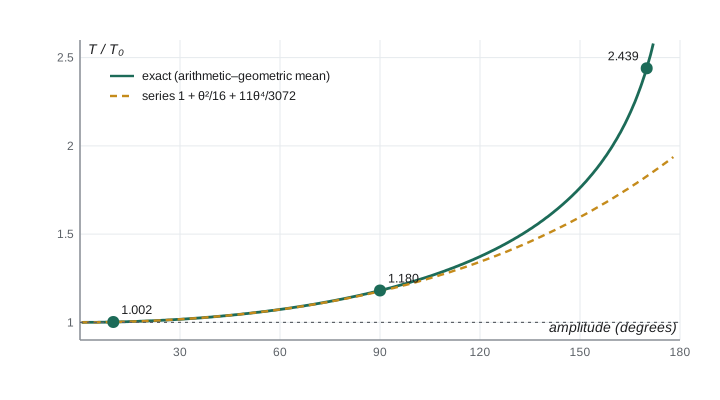
The figure shows the ratio \(T/T_0\). At \(10^\circ\) the period is only 0.19% longer than the small-angle value, which is why clockmakers could treat the pendulum as isochronous. At \(90^\circ\) it is 18% longer, and near \(170^\circ\) it is nearly two and a half times longer. The two-term series is a model error made visible: it is the right answer to a slightly different question, and its error grows with amplitude. The program below computes the period three ways and also integrates the equation of motion directly, which is what we would have to do if friction or a driving force were added and no formula existed at all.

import math

def agm(a, b, tol=1e-15):
    """Arithmetic-geometric mean; digits double each step."""
    steps = 0
    while abs(a - b) > tol * a:
        a, b = (a + b) / 2, math.sqrt(a * b)
        steps += 1
    return a, steps

def period_exact(theta0, L=1.0, g=9.81):
    T0 = 2 * math.pi * math.sqrt(L / g)
    m, steps = agm(1.0, math.cos(theta0 / 2))
    return T0 / m, steps

def period_series(theta0, L=1.0, g=9.81):
    T0 = 2 * math.pi * math.sqrt(L / g)
    return T0 * (1 + theta0**2 / 16 + 11 * theta0**4 / 3072)

def period_simulated(theta0, L=1.0, g=9.81, dt=1e-4):
    """Release from rest; time a quarter swing until theta crosses zero (RK4)."""
    def f(th, om): return om, -g / L * math.sin(th)
    th, om, t = theta0, 0.0, 0.0
    while True:
        k1 = f(th, om)
        k2 = f(th + dt/2 * k1[0], om + dt/2 * k1[1])
        k3 = f(th + dt/2 * k2[0], om + dt/2 * k2[1])
        k4 = f(th + dt * k3[0], om + dt * k3[1])
        th_new = th + dt/6 * (k1[0] + 2*k2[0] + 2*k3[0] + k4[0])
        om_new = om + dt/6 * (k1[1] + 2*k2[1] + 2*k3[1] + k4[1])
        if th_new <= 0:                      # crossed zero: interpolate the crossing time
            return 4 * (t + dt * th / (th - th_new))
        th, om, t = th_new, om_new, t + dt

T0 = 2 * math.pi * math.sqrt(1 / 9.81)
print(f"small-angle period T0 = {T0:.6f} s for L = 1 m")
print(" amp(deg)   exact T/T0   AGM steps   series T/T0   simulated T/T0")
for deg in (10, 30, 60, 90, 120, 150, 170):
    th = math.radians(deg)
    Te, n = period_exact(th)
    print(f"{deg:8d}   {Te/T0:10.6f}   {n:9d}   {period_series(th)/T0:11.6f}   {period_simulated(th)/T0:13.6f}")

small-angle period T0 = 2.006067 s for L = 1 m
 amp(deg)   exact T/T0   AGM steps   series T/T0   simulated T/T0
      10     1.001907           3      1.001907        1.001907
      30     1.017409           3      1.017404        1.017409
      60     1.073182           4      1.072845        1.073182
      90     1.180341           4      1.176012        1.180341
     120     1.372881           4      1.343054        1.372881
     150     1.762204           5      1.596576        1.762204
     170     2.439363           5      1.827724        2.439363

Three things stand out. The AGM needs only four or five steps for any amplitude short of the top, so the elliptic integral costs almost nothing. The series agrees with the exact value to six digits at \(10^\circ\) but is 9% low at \(150^\circ\). And the direct simulation, which knows nothing about elliptic integrals, matches the exact answer to every digit printed. When two independent methods agree, we have strong evidence that both are implemented correctly. This is verification by cross-checking, the most useful single habit in computational work.

The kinds of error

It is worth separating the errors carefully, because the remedies are different.

Modeling error is the gap between the mathematical model and nature. The point-mass pendulum ignores the size of the bob, the stretch of the string and the drag of the air. No amount of computing reduces modeling error; only better physics does. Data error comes from uncertain inputs. If the length is known to 1 mm in a meter, the period is uncertain by about 0.05%, whatever algorithm we use.

Discretization error, also called truncation error, comes from replacing continuous mathematics by finite approximations: a derivative by a difference quotient, an integral by a sum, a differential equation by a step-by-step recipe. It depends on a step size \(h\) and usually behaves like \(C h^p\) for small \(h\), where the integer \(p\) is the order of the method. Halving \(h\) divides the error of a first-order method by 2 and of a fourth-order method by 16. Much of this course is about designing methods with high order and about checking that a program achieves the order its method promises.

Round-off error comes from the finite precision of computer arithmetic. A double-precision number carries about 16 significant decimal digits, so every arithmetic operation may introduce a relative error of about \(10^{-16}\). Usually these errors are harmless, but some calculations amplify them enormously, as lesson 2 shows. Round-off sets a floor below which shrinking the step size makes results worse rather than better.

Finally there are mistakes: bugs in the program, wrong units, a sign error in a force. They are not small and they do not shrink with \(h\). The defenses are testing against known solutions, checking conservation laws, checking limiting cases, and comparing different methods.

Measuring the order of a method

If the error behaves like \(E(h) \approx C h^p\), then \(E(h)/E(h/2) \approx 2^p\), so

When the exact answer is known, we can compute \(E\) directly and read off \(p\). When it is not, we can still estimate \(p\) from three results at steps \(h\), \(h/2\) and \(h/4\): the differences between successive results shrink by the same factor \(2^p\). Measuring the observed order is the single most powerful test of a numerical code. A method that should be fourth order but shows order one has a bug, very often in the way a boundary condition or a time-dependent force is handled.

import math

f, df_exact, x = math.sin, math.cos(1.0), 1.0
print("    h        forward error   ratio    central error   ratio")
prev_f = prev_c = None
for k in range(1, 15):
    h = 10.0 ** (-k / 2)               # h = 0.316, 0.1, 0.0316, ...
    fwd = (f(x + h) - f(x)) / h
    cen = (f(x + h) - f(x - h)) / (2 * h)
    ef, ec = abs(fwd - df_exact), abs(cen - df_exact)
    rf = f"{prev_f / ef:6.2f}" if prev_f else "   -  "
    rc = f"{prev_c / ec:6.2f}" if prev_c else "   -  "
    print(f"{h:9.2e}   {ef:12.3e}   {rf}   {ec:12.3e}   {rc}")
    prev_f, prev_c = ef, ec
print("each step divides h by sqrt(10) = 3.16; order 1 gives ratio 3.16, order 2 gives 10")

    h        forward error   ratio    central error   ratio
 3.16e-01      1.409e-01      -        8.960e-03      -  
 1.00e-01      4.294e-02     3.28      9.001e-04     9.96
 3.16e-02      1.339e-02     3.21      9.005e-05    10.00
 1.00e-02      4.216e-03     3.18      9.005e-06    10.00
 3.16e-03      1.331e-03     3.17      9.005e-07    10.00
 1.00e-03      4.208e-04     3.16      9.005e-08    10.00
 3.16e-04      1.331e-04     3.16      9.005e-09    10.00
 1.00e-04      4.207e-05     3.16      9.004e-10    10.00
 3.16e-05      1.330e-05     3.16      8.893e-11    10.13
 1.00e-05      4.207e-06     3.16      1.114e-11     7.98
 3.16e-06      1.330e-06     3.16      6.005e-13    18.55
 1.00e-06      4.207e-07     3.16      2.772e-11     0.02
 3.16e-07      1.330e-07     3.16      1.815e-11     1.53
 1.00e-07      4.183e-08     3.18      1.943e-10     0.09
each step divides h by sqrt(10) = 3.16; order 1 gives ratio 3.16, order 2 gives 10

The forward difference loses a factor of about 3.16 each time \(h\) shrinks by \(\sqrt{10}\), so it is first order; the central difference loses a factor of about 10, so it is second order. Near the bottom of the table the central difference stops improving and starts to wander: round-off has taken over. Lesson 3 explains exactly where that turning point lies.

Cost, scale and choosing an algorithm

Accuracy is not the only consideration. An algorithm has a cost, usually counted in arithmetic operations or in evaluations of an expensive function such as a force. A fourth-order method that needs four force evaluations per step can still be far cheaper than a first-order method that needs one, because it reaches a given accuracy with vastly larger steps. Cost also depends on problem size \(N\): computing all pairwise gravitational forces among \(N\) bodies takes about \(N^2/2\) operations, solving a dense linear system takes about \(N^3/3\), and a fast Fourier transform of \(N\) samples takes about \(N \log_2 N\). Knowing these scalings tells you in advance whether a calculation will take a second or a century.

Stability is the third consideration. Some methods amplify small errors from step to step until the solution explodes, however accurate each step is on its own. Lesson 5 shows that the simple Euler method is unstable for an undamped oscillator at any step size, and lesson 8 shows that an explicit scheme for heat flow blows up unless the time step obeys a strict limit. Good algorithms are accurate, cheap and stable at once, and when they cannot be all three we must know which property we are giving up.

A little history

Numerical methods are older than computers. Newton's method for roots dates from the 1660s, Leonhard Euler described his stepping method for differential equations in 1768, and Carl Friedrich Gauss devised his quadrature rules in 1814. Astronomers computed planetary orbits by hand for two centuries; the discovery of Neptune in 1846 rested on long calculations by Urbain Le Verrier and John Couch Adams. In the 1940s the ENIAC computed artillery tables and, soon after, calculations for nuclear weapons design at Los Alamos, where Stanislaw Ulam and John von Neumann developed the Monte Carlo method between 1946 and 1949. In 1953 Enrico Fermi, John Pasta, Stanislaw Ulam and Mary Tsingou used the MANIAC computer to simulate a chain of masses joined by slightly nonlinear springs. They expected the energy to spread evenly among all the modes; instead it returned almost entirely to the starting mode, a surprise reported in 1955 that launched the study of nonlinear dynamics and solitons. Edward Lorenz's 1963 discovery of sensitive dependence on initial conditions also came from a computer simulation, of a simplified model of convection. Computation has been a source of new physics, not just a tool for confirming old physics.

Good habits

A few habits make computational work reliable. Use units consistently and print them. Start with a case whose answer you know, such as a small-angle pendulum or a free particle, and check the program reproduces it. Measure the order of convergence. Check conservation laws, such as energy for a frictionless system. Vary parameters that should not matter, such as the step size once converged, and confirm the answer does not change. Fix the seed of any random number generator so that results can be reproduced. Keep the code readable, with one function per idea, so that a reader can check it against the equations. These habits take a little time and save a great deal.