Partial differential equations: heat, wave and Laplace by finite differences

Fields that vary in both space and time obey partial differential equations: temperature in a cooling rod, displacement of a vibrating string, electric potential between conductors, the wave function of an electron, the pressure in a sound wave. Three equations serve as prototypes for almost all of them. The heat equation describes diffusion, the wave equation describes propagation and the Laplace equation describes equilibrium. This lesson discretizes each on a grid, using the difference formulas of lesson 3, and discovers that the choice of time step is governed not just by accuracy but by stability conditions with a clear physical meaning.

Three prototypes

In one space dimension the three equations are

They are called parabolic, hyperbolic and elliptic, by analogy with conic sections. The classification matters because it decides what information is needed and how it travels. A parabolic equation such as heat flow needs an initial temperature profile and boundary conditions, and every point immediately feels a disturbance anywhere, though only faintly at a distance. A hyperbolic equation needs an initial displacement and velocity, and disturbances travel at a finite speed \(c\). An elliptic equation has no time at all; the solution at every point depends on the boundary values all around, and it is found by solving everything at once.

We place grid points \(x_j = j\,\Delta x\) and, for time-dependent problems, time levels \(t_n = n\,\Delta t\), and write \(u_j^n\) for the approximation to \(u(x_j, t_n)\). The second derivative in space becomes the three-point formula \((u_{j+1} - 2u_j + u_{j-1})/\Delta x^2\) from lesson 3, accurate to \(O(\Delta x^2)\).

The heat equation: an explicit scheme

The simplest scheme uses a forward difference in time and the central difference in space, giving the forward-time centered-space or FTCS scheme:

Each new value is a weighted average of its old value and its two neighbors, which is diffusion in miniature. The scheme is explicit, easy to code, first order in time and second order in space. But it has a catch. John von Neumann's stability analysis, developed at Los Alamos in the 1940s, substitutes a single Fourier mode \(u_j^n = G^n e^{ikj\Delta x}\). The scheme multiplies each mode by the amplification factor

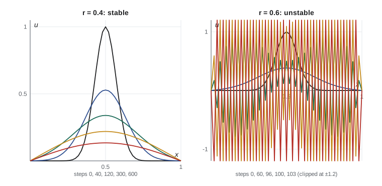
The true solution damps every mode, so we need \(|G| \le 1\) for all \(k\). The worst case is the shortest wavelength the grid can represent, \(k\Delta x = \pi\), where \(G = 1 - 4r\). Stability therefore requires

If \(r\) exceeds one half, the grid-scale zigzag mode is multiplied by a number less than \(-1\) every step: it flips sign and grows, and within a few dozen steps it swamps the solution. The condition is severe. Halving \(\Delta x\) for better spatial accuracy forces the time step down by a factor of four, so the total work for a given simulated time rises eightfold in one dimension.

Implicit schemes and the tridiagonal solver

Evaluating the spatial difference at the new time level instead gives the backward-time, or implicit, scheme

whose amplification factor \(G = 1/(1 + 4r\sin^2(k\Delta x/2))\) lies between 0 and 1 for every \(r\). It is unconditionally stable. The price is that each step requires solving a linear system for all the new values at once. The system is tridiagonal: each equation involves only a point and its two neighbors. Such systems are solved by Gaussian elimination specialized to three diagonals, the Thomas algorithm, named after Llewellyn Thomas, in about \(8N\) operations, as cheap as the explicit update itself.

John Crank and Phyllis Nicolson proposed in 1947 averaging the explicit and implicit schemes. The Crank–Nicolson scheme is second order in time as well as space and unconditionally stable, which makes it the standard choice for diffusion problems and, in a complex form, for the time-dependent Schrödinger equation, where it also preserves the total probability exactly. Its one weakness is that it damps the shortest wavelengths only weakly when \(r\) is large, so sharp initial features can leave a faint zigzag that decays slowly.

import math

L_rod, N, D = 1.0, 50, 1.0                     # rod of unit length, ends held at zero
dx = L_rod / N
x = [j * dx for j in range(N + 1)]
u0 = [math.sin(math.pi * xi) + 0.5 * math.sin(3 * math.pi * xi) for xi in x]
def exact(t):
    return [math.exp(-math.pi**2 * D * t) * math.sin(math.pi * xi)
            + 0.5 * math.exp(-9 * math.pi**2 * D * t) * math.sin(3 * math.pi * xi) for xi in x]

def ftcs(u, r, steps):
    u = u[:]
    for _ in range(steps):
        u = [0.0] + [u[j] + r * (u[j+1] - 2*u[j] + u[j-1]) for j in range(1, N)] + [0.0]
    return u

def thomas(a, b, c, d):
    """Solve a tridiagonal system: a sub-, b main, c super-diagonal, d right side."""
    n = len(d); cp, dp = [0.0] * n, [0.0] * n
    cp[0], dp[0] = c[0] / b[0], d[0] / b[0]
    for i in range(1, n):
        m = b[i] - a[i] * cp[i-1]
        cp[i] = c[i] / m if i < n - 1 else 0.0
        dp[i] = (d[i] - a[i] * dp[i-1]) / m
    out = [0.0] * n
    out[-1] = dp[-1]
    for i in range(n - 2, -1, -1):
        out[i] = dp[i] - cp[i] * out[i+1]
    return out

def crank_nicolson(u, r, steps):
    u = u[:]; n = N - 1
    a, b, c = [-r/2] * n, [1 + r] * n, [-r/2] * n
    for _ in range(steps):
        d = [r/2 * u[j-1] + (1 - r) * u[j] + r/2 * u[j+1] for j in range(1, N)]
        u = [0.0] + thomas(a, b, c, d) + [0.0]
    return u

T = 0.1
ex = exact(T)
def maxerr(u): return max(abs(u[j] - ex[j]) for j in range(N + 1))
for r in (0.25, 0.4, 0.5, 0.6):
    dt = r * dx * dx / D; steps = round(T / dt)
    print(f"FTCS            r = {r:4.2f}  dt = {dt:.2e}  steps = {steps:4d}  max error = {maxerr(ftcs(u0, r, steps)):.2e}")
for r in (0.5, 5.0, 50.0):
    dt = r * dx * dx / D; steps = round(T / dt)
    print(f"Crank-Nicolson  r = {r:4.1f}  dt = {dt:.2e}  steps = {steps:4d}  max error = {maxerr(crank_nicolson(u0, r, steps)):.2e}")

FTCS            r = 0.25  dt = 1.00e-04  steps = 1000  max error = 5.96e-05
FTCS            r = 0.40  dt = 1.60e-04  steps =  625  max error = 1.67e-04
FTCS            r = 0.50  dt = 2.00e-04  steps =  500  max error = 2.39e-04
FTCS            r = 0.60  dt = 2.40e-04  steps =  417  max error = 2.77e+43
Crank-Nicolson  r =  0.5  dt = 2.00e-04  steps =  500  max error = 1.19e-04
Crank-Nicolson  r =  5.0  dt = 2.00e-03  steps =   50  max error = 1.09e-04
Crank-Nicolson  r = 50.0  dt = 2.00e-02  steps =    5  max error = 1.01e-03

Below \(r = \frac12\) the explicit scheme is accurate to a few parts in \(10^4\) at time 0.1; at exactly one half it is still bounded; at 0.6 the error has reached \(10^{43}\) after about 400 steps. The initial profile contains no grid-scale zigzag at all: the instability grew from rounding errors of \(10^{-16}\), multiplied by \(|1 - 4r| = 1.4\) at every step. Crank–Nicolson with \(r = 5\) is as accurate as the explicit scheme at \(r = 0.5\) with a tenth of the steps, and even with \(r = 50\), a time step a hundred times beyond the explicit limit, five steps give an error of \(10^{-3}\). Stability does not guarantee accuracy, but it lets us choose the step for accuracy alone.

The wave equation and the CFL condition

For the wave equation, central differences in both time and space give the leapfrog scheme

which is second order in both. The dimensionless number \(C\) is the Courant number. Von Neumann's analysis shows that the scheme is stable if and only if \(C \le 1\). Richard Courant, Kurt Friedrichs and Hans Lewy identified this condition in 1928, years before electronic computers, and its meaning is physical. In one time step the true wave travels a distance \(c\,\Delta t\); the numerical scheme can only pass information one grid spacing per step. If \(c\,\Delta t > \Delta x\), the true solution at a point depends on initial data that the numerical scheme has not yet had time to see, and no scheme can be both explicit and correct. The domain of dependence of the numerical method must contain that of the equation.

The one-dimensional leapfrog scheme has a curious property at \(C = 1\): it is exact. The update then reduces to \(u_j^{n+1} = u_{j+1}^n + u_{j-1}^n - u_j^{n-1}\), which is satisfied exactly by any sum of left- and right-moving waves sampled on the grid, as d'Alembert's solution of 1747 shows. This magic time step is special to one dimension and constant wave speed, but it illustrates why waves are best computed with the largest stable step: smaller Courant numbers introduce numerical dispersion, in which short wavelengths travel too slowly and a sharp pulse sheds ripples behind it.

To start leapfrog we need two time levels. For a string released from rest, a Taylor expansion gives \(u_j^1 = u_j^0 + \frac{C^2}{2}(u_{j+1}^0 - 2u_j^0 + u_{j-1}^0)\). The program plucks a string of length 1 at a quarter of its length, the way a guitarist plucks near the bridge, and checks that after one full period \(2L/c\) the shape returns.

import math

N, c, Ltot = 100, 1.0, 1.0
dx = Ltot / N
pluck = 0.25
u0 = [(j * dx / pluck if j * dx <= pluck else (1 - j * dx) / (1 - pluck)) * 0.01
      for j in range(N + 1)]                     # 1 cm peak displacement

def run(C, periods=1.0):
    dt = C * dx / c
    steps = round(periods * 2 * Ltot / c / dt)
    prev = u0[:]
    cur = [0.0] + [u0[j] + C*C/2 * (u0[j+1] - 2*u0[j] + u0[j-1]) for j in range(1, N)] + [0.0]
    for _ in range(steps - 1):
        nxt = [0.0] + [2*cur[j] - prev[j] + C*C * (cur[j+1] - 2*cur[j] + cur[j-1])
                       for j in range(1, N)] + [0.0]
        prev, cur = cur, nxt
    return max(abs(cur[j] - u0[j]) for j in range(N + 1)), steps

for C in (1.0, 0.9, 0.5, 1.02):
    err, steps = run(C)
    tag = "  (unstable)" if err > 1 else ""
    print(f"Courant number {C:4.2f}: {steps:4d} steps, max difference from start after one period {err:.2e} m{tag}")

# frequencies of the modes the pluck excites: f_n = n c / (2L), amplitude of mode n
amps = [2 * sum(u0[j] * math.sin(n * math.pi * j * dx) for j in range(N + 1)) * dx for n in range(1, 9)]
print("mode amplitudes (mm):", " ".join(f"{1000 * a:+.3f}" for a in amps))
print("a pluck at L/4 leaves out every fourth harmonic: mode 4 and mode 8 are near zero")

Courant number 1.00:  200 steps, max difference from start after one period 8.67e-18 m
Courant number 0.90:  222 steps, max difference from start after one period 2.50e-04 m
Courant number 0.50:  400 steps, max difference from start after one period 3.55e-04 m
Courant number 1.02:  196 steps, max difference from start after one period 1.09e+28 m  (unstable)
mode amplitudes (mm): +7.643 +2.703 +0.850 -0.000 -0.306 -0.301 -0.157 +0.000
a pluck at L/4 leaves out every fourth harmonic: mode 4 and mode 8 are near zero

At \(C = 1\) the string returns to its starting shape to rounding error. At \(C = 0.9\) and \(0.5\) it returns approximately, with errors from numerical dispersion that grow as \(C\) decreases. At \(C = 1.02\), just 2% over the limit, the solution explodes. The mode amplitudes show physics that a guitarist uses: plucking at one quarter of the length gives no fourth or eighth harmonic, because those modes have a node exactly at the plucking point.

The Laplace equation and relaxation

In two dimensions, the five-point discretization of \(\nabla^2 u = 0\) on a square grid with spacing \(h\) says that each interior value is the average of its four neighbors:

This is the discrete form of the mean value property of harmonic functions, and it suggests an algorithm. Start with any guess, then repeatedly replace each interior value by the average of its neighbors, holding the boundary values fixed. This is Jacobi iteration, and it converges to the solution because it is equivalent to running the heat equation to its steady state with \(r = \frac14\), the largest stable value in two dimensions. Gauss–Seidel iteration uses each new value as soon as it is computed, which halves the number of iterations. Successive over-relaxation, or SOR, analyzed by David Young in his 1950 thesis, pushes each update further in the direction it was going: \(u \gets u + \omega(\bar u - u)\) with \(1 < \omega < 2\). With the optimal \(\omega = 2/(1 + \sin(\pi/N))\) for an \(N \times N\) grid, the number of iterations falls from order \(N^2\) to order \(N\).

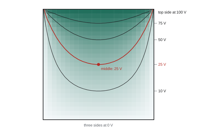
A neat test case has an exact answer. A square box has three sides grounded and the fourth held at 100 V. By superposition, adding the four rotated versions of this problem gives a box with all sides at 100 V, whose interior is at 100 V everywhere; by symmetry each version contributes equally at the center, so the center is at exactly 25 V.

import math

N = 24                                      # interior points per side
def solve(method, omega=1.0, tol=1e-6):
    u = [[0.0] * (N + 2) for _ in range(N + 2)]
    for j in range(N + 2):
        u[N + 1][j] = 100.0                    # top edge at 100 V
    u[N + 1][0] = u[N + 1][N + 1] = 0.0       # corners belong to the grounded sides
    for it in range(1, 20000):
        change = 0.0
        if method == "Jacobi":
            new = [row[:] for row in u]
            for i in range(1, N + 1):
                for j in range(1, N + 1):
                    new[i][j] = 0.25 * (u[i+1][j] + u[i-1][j] + u[i][j+1] + u[i][j-1])
                    change = max(change, abs(new[i][j] - u[i][j]))
            u = new
        else:
            for i in range(1, N + 1):
                for j in range(1, N + 1):
                    avg = 0.25 * (u[i+1][j] + u[i-1][j] + u[i][j+1] + u[i][j-1])
                    d = omega * (avg - u[i][j])
                    u[i][j] += d
                    change = max(change, abs(d))
        if change < tol:
            return u, it
    return u, it

w_opt = 2 / (1 + math.sin(math.pi / (N + 1)))
for name, method, w in (("Jacobi", "Jacobi", 1.0), ("Gauss-Seidel", "GS", 1.0),
                        ("SOR, omega = 1.5", "GS", 1.5), (f"SOR, omega = {w_opt:.3f}", "GS", w_opt)):
    u, its = solve(method, w)
    mid = (u[N//2][N//2] + u[N//2+1][N//2] + u[N//2][N//2+1] + u[N//2+1][N//2+1]) / 4
    print(f"{name:22s} {its:5d} iterations   potential at the middle of the box {mid:.4f} V")
print("exact value at the middle: 25 V (by superposition and symmetry)")

Jacobi                  1602 iterations   potential at the middle of the box 24.9999 V
Gauss-Seidel             852 iterations   potential at the middle of the box 24.9999 V
SOR, omega = 1.5         304 iterations   potential at the middle of the box 25.0000 V
SOR, omega = 1.777        90 iterations   potential at the middle of the box 25.0000 V
exact value at the middle: 25 V (by superposition and symmetry)

Jacobi needs well over a thousand sweeps, Gauss–Seidel about half as many, and SOR with the optimal factor fewer than a hundred. All agree that the middle of the box is at 25 V. The discrete equations obey the same superposition argument as the continuous ones, so the exact discrete answer at the middle is also 25 V, and the tiny remaining differences come from the iteration tolerance alone. That makes this a clean test of the solver rather than of the discretization. For large grids even SOR becomes slow, and modern codes use multigrid methods, which solve the problem on a hierarchy of coarser grids and need only a fixed number of sweeps however fine the grid, or fast Fourier transform solvers for simple geometries.