Ordinary differential equations: Euler, Runge–Kutta and adaptive steps

Newton's second law is a differential equation, and so are the laws of radioactive decay, chemical kinetics, electrical circuits and population dynamics. Given the state of a system now, the equation says how fast the state is changing, and the task is to march forward in time. This lesson develops the standard marching methods, from Euler's simple step to the classical fourth-order Runge–Kutta method, and shows how to choose the step size automatically so that the solution is accurate where it changes quickly and cheap where it changes slowly. Along the way it introduces stability, which decides whether small errors stay small.

Reducing to a first-order system

Every method in this lesson solves a system of first-order equations

where \(\mathbf{y}\) is a list of numbers describing the state. A second-order equation such as \(m\ddot x = F(x, \dot x, t)\) becomes first order by introducing the velocity as a separate variable: with \(\mathbf{y} = (x, v)\), the system is \(\dot x = v\), \(\dot v = F/m\). A projectile in two dimensions has the four-component state \((x, y, v_x, v_y)\); \(N\) gravitating bodies in three dimensions have \(6N\) components. Once the problem is in this form, one integrator handles them all, and in Python the state can be a plain list.

Euler's method

The simplest idea is to assume the rate of change stays constant over a short step \(h\):

Leonhard Euler described this in his Institutiones calculi integralis of 1768. Comparing with the Taylor expansion \(\mathbf{y}(t + h) = \mathbf{y}(t) + h\mathbf{y}'(t) + \frac{h^2}{2}\mathbf{y}''(\xi)\) shows that each step makes a local error of order \(h^2\). To cross a fixed interval \(T\) takes \(T/h\) steps, and if the local errors accumulate without much amplification the global error is of order \(T/h \times h^2 = Th\). Euler's method is therefore first order: halving the step halves the error. It is easy to understand and easy to program, and almost never the right choice for serious work.

Stability and the harmonic oscillator

Accuracy over one step is not the whole story. Apply Euler's method to the test equation \(y' = \lambda y\), whose exact solution \(e^{\lambda t}\) decays when \(\lambda < 0\). One step multiplies \(y\) by \(1 + h\lambda\). The numerical solution decays only if \(|1 + h\lambda| < 1\), that is \(h < 2/|\lambda|\). A step larger than that produces an oscillating, growing solution of an equation whose true solution decays smoothly: the method is unstable. Germund Dahlquist built the modern theory of such stability conditions in the 1950s.

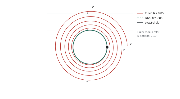
The harmonic oscillator \(\ddot x = -\omega^2 x\) is worse. In complex form it corresponds to \(\lambda = \pm i\omega\), and Euler's amplification factor has magnitude \(|1 + ih\omega| = \sqrt{1 + h^2\omega^2} > 1\) for every \(h\). The energy grows by a factor \(1 + h^2\omega^2\) at every step, so the orbit in phase space spirals outward and the energy grows without limit, however small the step. With \(\omega = 1\) and \(h = 0.01\), the energy has grown by about 87% after ten periods. For a physicist this is a qualitative failure: a conservative system acquires energy from nowhere.

Runge–Kutta methods

Carl Runge suggested in 1895 that higher accuracy could be reached without computing higher derivatives by evaluating \(\mathbf{f}\) at several trial points within each step and combining the slopes cleverly. The simplest example is the midpoint method: take a half step with Euler's slope, evaluate the slope there, and use it for the whole step,

Expanding in Taylor series shows that the \(h^2\) error terms cancel, so the method is second order. Karl Heun gave a related second-order method in 1900, and Martin Kutta in 1901 derived the four-stage scheme now called the classical Runge–Kutta method, or simply RK4:

Its local error is of order \(h^5\) and its global error of order \(h^4\). For a problem with no dependence on \(\mathbf{y}\), RK4 reduces to Simpson's rule applied to \(\int f\,dt\), which is one way to remember the weights \(1, 2, 2, 1\) over 6. RK4 costs four evaluations of \(\mathbf{f}\) per step, four times as many as Euler, but because its error falls so much faster it is far cheaper for any useful accuracy. To reach an error of \(10^{-6}\) on an oscillator over ten periods, Euler would need tens of millions of steps; RK4 needs a few hundred.

For the harmonic oscillator RK4's amplification factor is the Taylor polynomial \(1 + z + z^2/2 + z^3/6 + z^4/24\) with \(z = ih\omega\), whose magnitude is \(\sqrt{1 - (h\omega)^6/72 + (h\omega)^8/576}\). This is slightly less than 1 for \(h\omega < 2\sqrt2\), so RK4 loses energy very slowly, by about \((h\omega)^6/72\) of its value per step. For long simulations of conservative systems even that slow drift matters, and lesson 6 introduces symplectic methods that avoid it altogether.

import math

def f(t, y):                      # harmonic oscillator, omega = 1: y = [x, v]
    return [y[1], -y[0]]

def euler(f, t, y, h):
    k = f(t, y)
    return [y[i] + h * k[i] for i in range(len(y))]

def midpoint(f, t, y, h):
    k1 = f(t, y)
    k2 = f(t + h/2, [y[i] + h/2 * k1[i] for i in range(len(y))])
    return [y[i] + h * k2[i] for i in range(len(y))]

def rk4(f, t, y, h):
    n = len(y)
    k1 = f(t, y)
    k2 = f(t + h/2, [y[i] + h/2 * k1[i] for i in range(n)])
    k3 = f(t + h/2, [y[i] + h/2 * k2[i] for i in range(n)])
    k4 = f(t + h, [y[i] + h * k3[i] for i in range(n)])
    return [y[i] + h/6 * (k1[i] + 2*k2[i] + 2*k3[i] + k4[i]) for i in range(n)]

def solve(step, N, T):
    h, t, y = T / N, 0.0, [1.0, 0.0]
    for _ in range(N):
        y = step(f, t, y, h); t += h
    return y

T = 20 * math.pi                  # ten periods; exact answer x = 1, v = 0
print("   h       Euler error   midpoint error   RK4 error     RK4 energy")
prev = None
for N in (300, 600, 1200, 2400, 4800):
    h, errs = T / N, []
    for step in (euler, midpoint, rk4):
        x, v = solve(step, N, T)
        errs.append(math.hypot(x - 1.0, v))
    E = 0.5 * (x * x + v * v)
    print(f"{h:7.4f}   {errs[0]:11.3e}   {errs[1]:12.3e}   {errs[2]:11.3e}   {E:.10f}")
    if prev:
        print("         ratios " + "   ".join(f"{p / e:6.2f}" for p, e in zip(prev, errs)))
    prev = errs

   h       Euler error   midpoint error   RK4 error     RK4 energy
 0.2094     6.255e+02      4.718e-01     1.007e-03   0.4998251575
 0.1047     2.539e+01      1.153e-01     6.296e-05   0.4999945127
         ratios  24.63     4.09    15.99
 0.0524     4.171e+00      2.872e-02     3.935e-06   0.4999998283
         ratios   6.09     4.01    16.00
 0.0262     1.276e+00      7.178e-03     2.460e-07   0.4999999946
         ratios   3.27     4.00    16.00
 0.0131     5.086e-01      1.794e-03     1.537e-08   0.4999999998
         ratios   2.51     4.00    16.00

Each halving of \(h\) divides the RK4 error by about 16 and the midpoint error by about 4, confirming orders 4 and 2. Euler's error is not even small: at \(h = 0.2\) its error exceeds the size of the solution, because the spiral of the figure has carried it far from the circle. Halving the step eventually halves Euler's error, as first order predicts, but only once the step is small enough. The energy column shows RK4's slow loss: with \(h \approx 0.2\) the energy after ten periods is down by about 0.035%, in line with the estimate \((h\omega)^6/72\) per step, and with smaller steps the loss quickly becomes invisible.

Adaptive step-size control

A fixed step is wasteful when the solution changes quickly at some times and slowly at others: a comet near perihelion moves hundreds of times faster than near aphelion, and a fixed step small enough for the first is absurdly small for the second. Adaptive methods estimate the local error of each step and adjust \(h\) to keep it near a tolerance.

The simplest estimate is step doubling. Take one RK4 step of size \(h\) to get \(\mathbf{y}_1\), and two steps of size \(h/2\) to get \(\mathbf{y}_2\). Both have local errors proportional to \(h^5\), and the second is smaller by a factor of about 16, so \(\Delta = |\mathbf{y}_2 - \mathbf{y}_1|/15\) estimates the error of \(\mathbf{y}_2\). If \(\Delta\) exceeds the tolerance \(\tau\) the step is rejected and retried with a smaller \(h\). Either way the next step size is chosen as

since the local error scales as \(h^5\); the safety factor 0.9 avoids repeated rejections. The extrapolated value \(\mathbf{y}_2 + (\mathbf{y}_2 - \mathbf{y}_1)/15\) is even more accurate, which is Richardson's idea again. Production codes use embedded Runge–Kutta pairs instead, in which a fourth-order and a fifth-order result share the same stages so that the error estimate costs almost nothing extra. Erwin Fehlberg published such pairs in 1969, and the pair of John Dormand and Peter Prince from 1980 is the default in many libraries.

A projectile with air resistance

A baseball does not fly in a parabola. At the speeds of a hard hit, air drag is roughly proportional to the square of the speed, \(\mathbf{F}_D = -\frac12\rho C_D A\,|\mathbf{v}|\mathbf{v}\), where \(\rho \approx 1.2\) kg per cubic meter is the density of air, \(A\) the cross-sectional area and \(C_D \approx 0.35\) the drag coefficient. The equations of motion,

have no closed-form solution in two dimensions. For a baseball of mass 0.145 kg and diameter 7.4 cm, \(k \approx 0.0062\) per meter. The program integrates the trajectory with adaptive RK4 by step doubling, finds the landing point by interpolating between the last two steps, and compares the range with the vacuum value \(v_0^2\sin 2\theta/g\).

import math

g, rho, Cd, m, d = 9.81, 1.2, 0.35, 0.145, 0.074
k = rho * Cd * math.pi * (d / 2) ** 2 / (2 * m)

def f(t, s):
    x, y, vx, vy = s
    sp = math.hypot(vx, vy)
    return [vx, vy, -k * sp * vx, -g - k * sp * vy]

def rk4(t, s, h):
    def add(a, b, c): return [a[i] + c * b[i] for i in range(4)]
    k1 = f(t, s); k2 = f(t + h/2, add(s, k1, h/2))
    k3 = f(t + h/2, add(s, k2, h/2)); k4 = f(t + h, add(s, k3, h))
    return [s[i] + h/6 * (k1[i] + 2*k2[i] + 2*k3[i] + k4[i]) for i in range(4)]

def fly(v0, deg, tol=1e-8):
    th = math.radians(deg)
    t, s, h = 0.0, [0.0, 0.0, v0 * math.cos(th), v0 * math.sin(th)], 0.1
    steps = rejected = 0
    while True:
        big = rk4(t, s, h)
        half = rk4(t + h/2, rk4(t, s, h/2), h/2)
        err = max(abs(half[i] - big[i]) for i in range(4)) / 15
        if err > tol:
            h *= max(0.2, 0.9 * (tol / err) ** 0.2); rejected += 1; continue
        new = [half[i] + (half[i] - big[i]) / 15 for i in range(4)]
        if new[1] < 0:                           # crossed the ground: interpolate
            frac = s[1] / (s[1] - new[1])
            return s[0] + frac * (new[0] - s[0]), t + frac * h, steps, rejected
        t, s, steps = t + h, new, steps + 1
        h *= min(5.0, 0.9 * (tol / max(err, 1e-300)) ** 0.2)

print(f"drag constant k = {k:.5f} per m")
v0 = 45.0
print(" angle   vacuum range   range with drag   flight time   steps  rejected")
for deg in (20, 30, 35, 40, 45, 50):
    R0 = v0**2 * math.sin(2 * math.radians(deg)) / g
    R, T, n, r = fly(v0, deg)
    print(f"{deg:5d}   {R0:10.1f} m   {R:13.1f} m   {T:9.2f} s   {n:5d}  {r:7d}")
best = max(range(200, 500), key=lambda a: fly(v0, a / 10)[0])
print(f"best angle with drag about {best / 10:.1f} degrees")

drag constant k = 0.00623 per m
 angle   vacuum range   range with drag   flight time   steps  rejected
   20        132.7 m            87.8 m        2.79 s      23        1
   30        178.8 m           105.5 m        3.92 s      30        1
   35        194.0 m           109.6 m        4.43 s      34        1
   40        203.3 m           111.1 m        4.90 s      37        1
   45        206.4 m           109.9 m        5.34 s      40        1
   50        203.3 m           106.3 m        5.74 s      43        1
best angle with drag about 39.8 degrees

Drag cuts the range of a well-hit ball nearly in half, and the best launch angle falls below the vacuum value of \(45^\circ\), because a lower trajectory spends less time fighting the air. The adaptive integrator takes only a few dozen steps per flight to reach a tolerance of \(10^{-8}\). Real baseballs are more complicated still: the drag coefficient changes with speed as the boundary layer becomes turbulent, and backspin adds a lift force, the Magnus effect, which lets a hit ball carry farther than this model predicts. Adding those effects means adding terms to \(\mathbf{f}\); the integrator does not change.

Stiff equations

Some systems contain processes on wildly different time scales: a chemical reaction network with rates differing by a factor of a million, or a circuit with a tiny capacitor beside a large one. The fast processes decay almost instantly, but explicit methods such as Euler and RK4 must still use steps small enough to keep them stable, \(h \lesssim 2/|\lambda_{\text{fast}}|\), long after they have died away. Such problems are called stiff, a term introduced by Charles Curtiss and Joseph Hirschfelder in 1952. They are solved with implicit methods such as backward Euler, \(\mathbf{y}_{n+1} = \mathbf{y}_n + h\mathbf{f}(t_{n+1}, \mathbf{y}_{n+1})\), whose amplification factor \(1/(1 - h\lambda)\) has magnitude below 1 for every \(h\) when \(\lambda < 0\). Each step requires solving an equation, often by Newton's method, but the steps can be enormous. Lesson 8 meets the same idea for the heat equation.