
NUC-320 · Lesson 5 of 12 · 23 min
Gamma shielding and buildup
Hana's first shielding calculation for Meridian Nuclear Engineering's design group goes wrong in an instructive way. She sizes a concrete wall for a resin storage room using the narrow-beam formula from lesson 4, and Dr. Vasquez sends it back with one word circled: buildup. The wall is thick enough for a pencil beam of photons traveling straight through, but not for the real situation, in which many photons scatter inside the wall and still reach the other side. This lesson explains what she missed and how shielding engineers correct for it.
How photons interact in a shield
A gamma photon crossing matter can be removed from its path in three main ways. In the photoelectric effect it is absorbed completely by an atom, which ejects an electron; this dominates at low energies and in high-Z materials such as lead. In Compton scattering it gives part of its energy to an electron and continues in a new direction with less energy; this dominates in most materials between about 0.1 and 5 MeV, the range of most reactor and industrial gamma rays. In pair production, possible above 1.022 MeV and important only at several MeV, the photon converts to an electron and positron near a nucleus, and the positron later annihilates into two 0.511 MeV photons.
The probabilities of these processes add to give the linear attenuation coefficient \(\mu\), in cm⁻¹. Because they depend on the electron density and atomic number, it is convenient to divide by density to obtain the mass attenuation coefficient \(\mu/\rho\), in cm²/g, which varies much less between materials in the Compton region. At about 1 MeV, \(\mu/\rho\) is close to 0.06 to 0.07 cm²/g for almost everything from water to iron, so a gram per square centimeter of concrete stops about as many photons as a gram per square centimeter of steel. Lead is better at lower energies because of its strong photoelectric absorption.
| Material | Density (g/cm³) | µ at 0.662 MeV (cm⁻¹) | µ at 1.25 MeV (cm⁻¹) |
|---|---|---|---|
| Water | 1.00 | 0.086 | 0.063 |
| Ordinary concrete | 2.3 | 0.18 | 0.13 |
| Steel | 7.9 | 0.58 | 0.43 |
| Lead | 11.35 | 1.25 | 0.67 |
Narrow beam and broad beam
The simple exponential law \(I = I_0 e^{-\mu x}\) describes a narrow, well-collimated beam measured by a small detector far behind the shield. Any photon that interacts is removed from the beam and does not reach the detector. Real shielding geometry is different. A source radiates in all directions, the shield is wide, and the person behind it is a large target. Photons that Compton scatter in the shield often continue roughly forward and reach the person, with reduced energy but still contributing dose. The dose behind a real shield is therefore greater than the narrow-beam formula predicts.
Shielding engineers correct for this with a dose buildup factor \(B\), always at least 1, so that the dose rate behind a shield from a point source becomes
The product \(\mu x\) is the shield thickness in mean free paths, the natural measure of how thick a shield is for photons. The buildup factor depends on the photon energy, the shield material, the geometry and the dose quantity. It grows with thickness, because a thicker shield has more scattering. For low-Z materials such as water and concrete it can be large, because Compton scattering dominates and scattered photons survive; for lead at low energy it is smaller, because scattered photons, now at lower energy, are quickly absorbed photoelectrically.
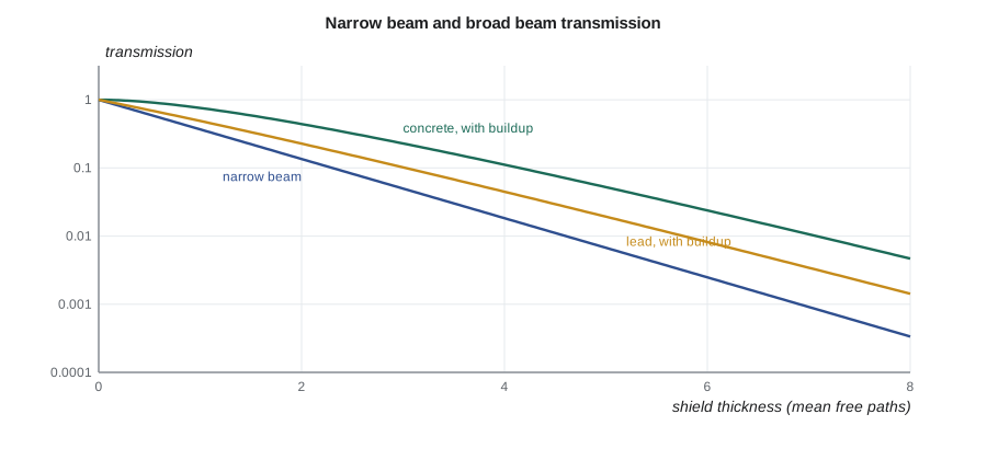
Representing buildup
Buildup factors are tabulated from transport calculations, most widely in the American Nuclear Society standard ANSI/ANS-6.4.3 and its successors, as functions of energy and mean free paths for common materials. For hand calculations they are often fitted with simple formulas. Two common forms are the Taylor form, a sum of two exponentials, and the Berger form
with coefficients \(a\) and \(b\) fitted for each material and energy. A useful rough rule for low-Z materials near 1 MeV is that \(B\) is a little more than \(1 + \mu x\) for moderate thicknesses. The coefficients in this lesson's program are illustrative values chosen to reproduce the general behavior; real designs use the tabulated data or a qualified code.
Worked problem
Hana's wall, with and without buildup
A point source gives 20 mSv/h at 2 m from cobalt-60 in spent resin. A concrete wall 50 cm thick lies between the source and an office. Using µ = 0.13 cm⁻¹ and an illustrative concrete buildup with a = 1.0 and b = 0.06, find the dose rate beyond the wall.
Show solution
- Mean free paths: \(\mu x = 0.13 \times 50 = 6.5\).
- Narrow beam: \(20 \times e^{-6.5} = 20 \times 1.50 \times 10^{-3} = 0.030\) mSv/h.
- Buildup: \(B = 1 + 1.0 \times 6.5 \times e^{0.39} = 1 + 6.5 \times 1.48 = 10.6\).
- Broad beam: \(0.030 \times 10.6 = 0.32\) mSv/h.
Answer: About 0.3 mSv/h, ten times Hana's first answer. The wall must be considerably thicker, as the program shows by solving for the thickness that meets a target.
# Gamma shielding with an illustrative Berger-form buildup factor B = 1 + a*mx*exp(b*mx).
import math
MU = {'concrete': 0.13, 'lead': 0.67, 'steel': 0.43}          # 1/cm at 1.25 MeV (approximate)
BERGER = {'concrete': (1.0, 0.06), 'lead': (0.32, 0.03), 'steel': (0.8, 0.05)}   # illustrative

def transmission(mat, x_cm, buildup=True):
    mx = MU[mat] * x_cm
    t = math.exp(-mx)
    if buildup:
        a, b = BERGER[mat]
        t *= 1 + a * mx * math.exp(b * mx)
    return t

H0 = 20.0   # mSv/h at the dose point with no shield
x = 50.0
print(f"50 cm concrete: {MU['concrete']*x:.1f} mean free paths")
print(f"  narrow beam {H0*transmission('concrete', x, False):.3f} mSv/h")
print(f"  with buildup {H0*transmission('concrete', x):.3f} mSv/h")

def thickness(mat, H0, target, buildup=True):
    lo, hi = 0.0, 500.0
    for _ in range(60):                     # bisection on thickness
        mid = (lo + hi) / 2
        if H0 * transmission(mat, mid, buildup) > target: lo = mid
        else: hi = mid
    return hi

target = 0.0025   # mSv/h (2.5 uSv/h) design target in the occupied area
for mat in ('concrete', 'steel', 'lead'):
    xn = thickness(mat, H0, target, False); xb = thickness(mat, H0, target, True)
    print(f"{mat:8s}: {xn:6.1f} cm without buildup, {xb:6.1f} cm with buildup (+{xb-xn:4.1f} cm)")

# Two layers: 5 cm lead (outer) plus concrete; buildup of the outer material at the total mfp
def two_layer(x_conc, x_lead):
    mx = MU['concrete'] * x_conc + MU['lead'] * x_lead
    a, b = BERGER['lead']
    return math.exp(-mx) * (1 + a * mx * math.exp(b * mx))
print(f"60 cm concrete + 5 cm lead outside: {H0*two_layer(60, 5)*1000:.2f} uSv/h (outer-layer buildup rule)")50 cm concrete: 6.5 mean free paths narrow beam 0.030 mSv/h with buildup 0.319 mSv/h concrete: 69.1 cm without buildup, 94.4 cm with buildup (+25.2 cm) steel : 20.9 cm without buildup, 27.7 cm with buildup (+ 6.8 cm) lead : 13.4 cm without buildup, 16.0 cm with buildup (+ 2.6 cm) 60 cm concrete + 5 cm lead outside: 1.72 uSv/h (outer-layer buildup rule)
Solving for a required thickness
Design usually runs the other way: the source and the target dose rate are known and the thickness is wanted. Without buildup, the answer is direct: \(x = \ln(\dot{H}_0/\dot{H}_{\text{target}})/\mu\). With buildup the equation cannot be solved in closed form, because \(B\) depends on \(x\). The simple method is iteration: guess the narrow-beam thickness, compute \(B\), add enough thickness to absorb it, and repeat until the change is small. The program does this with a bisection search. Each factor of 10 that buildup introduces costs about one TVL, which for cobalt-60 in concrete is roughly 20 cm.
Several layers
Many shields combine materials: a steel liner and concrete, or lead and steel in a transport cask. For narrow-beam attenuation the exponents simply add, \(e^{-(\mu_1 x_1 + \mu_2 x_2)}\). Buildup for layered shields is harder, because the spectrum of scattered photons depends on the order of the layers. Practical rules of thumb are to use the buildup factor of the outermost material evaluated at the total number of mean free paths, which is reasonable when the outer layer is thick, or to use the larger of the two materials' buildup factors as a conservative estimate. When a high-Z layer is placed on the outside, it absorbs many of the low-energy scattered photons that build up in a concrete layer, which is one reason lead linings are sometimes placed on the occupied side.
Energy matters
Shield thickness depends strongly on photon energy. Cesium-137 at 0.662 MeV needs roughly 40 % less concrete than cobalt-60 at 1.25 MeV for the same attenuation, and high-energy photons such as the 2.75 MeV line of sodium-24 or the 6 to 7 MeV gamma rays from nitrogen-16 in reactor coolant need much more. Nitrogen-16, produced from oxygen in the coolant by fast neutrons, is why the steam generator and coolant pump rooms of a running reactor need heavy shielding even though the activity decays within seconds of shutdown.
In a pressurized water reactor the reactor coolant system carries nitrogen-16 during operation, so containment is not entered for routine work at power, and shielding around the steam generators and pressurizer is designed for these high-energy photons.
Streaming, ducts and skyshine
A wall is only as good as its weakest path. Penetrations for pipes, cables and ventilation ducts allow radiation to stream through. Designers use offset or stepped penetrations, bends in ducts, shadow shields and labyrinth entrances so that radiation must scatter several times, losing energy and intensity each time, before reaching an occupied area. Gaps around doors and at joints between shield blocks are classic sources of hot spots found in surveys.
Radiation can also travel up over a shield wall and scatter back down from the air above, a process called skyshine. It matters for open-top shields around strong sources, such as storage pads and some accelerator facilities, and is usually controlled with a roof or a higher wall. Lesson 12 returns to penetrations and skyshine in the design project.
Materials and practicalities
| Material | Advantages | Drawbacks |
|---|---|---|
| Lead | thin; excellent at low energy; flexible blankets and bricks | heavy, soft, toxic; creeps; poor for neutrons |
| Steel | structural; good for high-energy photons | expensive per unit attenuation; activation products if near a reactor |
| Ordinary concrete | cheap; structural; contains hydrogen for neutrons | thick; density and water content vary |
| High-density concrete | iron or barite aggregate, thinner walls | cost; quality control of density |
| Water | transparent, cheap, cools; good for neutrons | thick; must be contained and its chemistry controlled |
For temporary shielding at a station, lead blankets and bricks dominate because they are compact and portable, but their weight must be checked against the strength of the pipe or support they hang from, and lead handling needs its own industrial hygiene controls. Permanent shielding is usually concrete because it is structural and cheap. Density must be confirmed during construction; a wall poured at 2.1 g/cm³ instead of the specified 2.35 provides about 10 % fewer mean free paths.
Checking a shield in the field
After a shield is installed, its performance is checked by measurement, and a simple check uses the attenuation law backwards. If the dose rate in front of a lead blanket is 1.6 mSv/h and behind it 0.45 mSv/h at the same distance, the effective attenuation is \(\ln(1.6/0.45) = 1.27\) mean free paths. For cobalt-60 in lead with µ = 0.67 cm⁻¹, that corresponds to about 1.9 cm of lead including buildup effects, which can be compared with the blanket's rated lead equivalence. A shield that attenuates much less than expected may have gaps, sagging or the wrong rating, or there may be another source contributing behind it.
Field checks also catch the most common error in temporary shielding, which is the assumption that a blanket rated for one energy works equally well at another. A blanket rated as 1.3 cm lead equivalent for the 0.662 MeV line of cesium-137 provides noticeably fewer mean free paths for the 1.25 MeV photons of cobalt-60, because µ for lead falls by almost half between those energies. Protection staff therefore record which nuclide dominates the field before choosing shielding, and use the coefficients for that energy when estimating the benefit.
Worked problem
Lead blanket at two energies
A 1.3 cm lead blanket is placed over a pipe. Using narrow-beam values, compare its transmission for Cs-137 (µ = 1.25 cm⁻¹) and Co-60 (µ = 0.67 cm⁻¹).
Show solution
- Cs-137: \(e^{-1.25 \times 1.3} = e^{-1.63} = 0.20\).
- Co-60: \(e^{-0.67 \times 1.3} = e^{-0.87} = 0.42\), before buildup.
Answer: The blanket cuts a cesium-137 field to about a fifth but a cobalt-60 field only to about two fifths, and buildup makes the real cobalt-60 transmission higher still.
Summary and key terms
- Photons interact by the photoelectric effect, Compton scattering and pair production; Compton dominates between about 0.1 and 5 MeV.
- Narrow-beam attenuation is e^{−µx}; real shields transmit more because of scattered photons.
- The buildup factor B(µx) ≥ 1 corrects for scatter; it is large for thick low-Z shields.
- Required thickness is found by iteration when buildup is included.
- Layered shields need care with buildup; penetrations, gaps and skyshine are common weak points.
- Shield thickness depends strongly on photon energy; nitrogen-16 drives operating reactor shielding.
- Linear attenuation coefficient
- Probability per unit length that a photon interacts, in cm⁻¹.
- Mass attenuation coefficient
- µ/ρ, in cm²/g, nearly the same for many materials in the Compton region.
- Mean free path
- Average distance a photon travels before interacting, 1/µ.
- Buildup factor
- Ratio of total dose behind a shield to the dose from unscattered photons alone.
- Streaming
- Radiation passing through gaps, ducts or penetrations in a shield.
- Skyshine
- Radiation scattered back to the ground from the air above an open shield.
Practice problems
Work each problem on paper first, then reveal the answer to check.
A shield is 4 mean free paths thick. What is the narrow-beam transmission?
Show answer
e⁻⁴ = 0.018.
With B = 5 at 4 mean free paths, what is the broad-beam transmission?
Show answer
0.092.
Why is buildup larger in concrete than in lead at 1 MeV?
Show answer
Compton-scattered photons survive in low-Z concrete but are absorbed photoelectrically in lead.
Roughly how much extra concrete does a buildup factor of 10 cost for Co-60?
Show answer
About one TVL, roughly 20 cm.
Name two ways to stop streaming through a duct.
Show answer
Bends or offsets in the duct, shadow shields, or a labyrinth.
Why do operating reactor coolant rooms need heavy shielding?
Show answer
Nitrogen-16 in the coolant emits 6 to 7 MeV gamma rays.
Lesson quiz · 5 questions
Score 60% or more to complete this lesson.
Create a free account to save your progress, take quizzes and earn a certificate.