Gauss's Theorema Egregium and isometries

Gaussian curvature was defined in lesson 8 as the determinant of the shape operator, a quantity built from the normal vector and therefore, it would seem, from how the surface sits in space. Gauss's great discovery was that it is nothing of the kind. This lesson proves that \(K\) can be computed from the first fundamental form alone, so that it is preserved by isometries and can be measured by an inhabitant of the surface. The proof uses the Christoffel symbols, which express second derivatives of a parametrization in terms of the frame \(\mathbf{x}_u, \mathbf{x}_v, N\), and it leads to explicit formulas, Brioschi's for general coordinates and a simpler one for orthogonal coordinates. The lesson closes with consequences: the impossibility of perfect maps, the bending of a helicoid into a catenoid, and Bonnet's theorem that the two fundamental forms determine a surface.

Christoffel symbols

At each point of a patch, the vectors \(\mathbf{x}_u, \mathbf{x}_v, N\) form a basis of \(\mathbb{R}^3\), so the second derivatives of \(\mathbf{x}\) can be expanded in it. The normal components are the coefficients of the second fundamental form, and the tangential coefficients are given names:

The six functions \(\Gamma^k_{ij}\) are the Christoffel symbols, introduced by Elwin Bruno Christoffel in 1869 in his work on quadratic differential forms; we set \(\Gamma^k_{21} = \Gamma^k_{12}\). Together with the Weingarten equations of lesson 7 for \(N_u\) and \(N_v\), these describe how the moving frame changes, exactly as the Frenet–Serret equations do for curves.

Lemma. The Christoffel symbols depend only on \(E\), \(F\), \(G\) and their first derivatives.

Proof. Take dot products of the three equations with \(\mathbf{x}_u\) and \(\mathbf{x}_v\); the \(N\) terms disappear. The left sides are computed by differentiating the coefficients of the first fundamental form:

For instance \(E_u = 2\langle \mathbf{x}_{uu}, \mathbf{x}_u \rangle\), and \(F_u = \langle \mathbf{x}_{uu}, \mathbf{x}_v \rangle + \langle \mathbf{x}_u, \mathbf{x}_{uv} \rangle = \langle \mathbf{x}_{uu}, \mathbf{x}_v \rangle + \frac12 E_v\). So each pair of Christoffel symbols with the same lower indices satisfies a linear system whose matrix is the Gram matrix; for example \(\Gamma^1_{11}E + \Gamma^2_{11}F = \frac12E_u\) and \(\Gamma^1_{11}F + \Gamma^2_{11}G = F_u - \frac12E_v\). The determinant \(EG - F^2\) is positive, so each system has a unique solution expressed through \(E, F, G\) and their first derivatives. \(\blacksquare\)

For an orthogonal parametrization, \(F = 0\), the systems decouple and give

On the plane in polar coordinates \((r, \theta)\), with \(E = 1\), \(F = 0\), \(G = r^2\), the only nonzero symbols are \(\Gamma^2_{12} = 1/r\) and \(\Gamma^1_{22} = -r\). They are not zero although the plane is flat: Christoffel symbols describe the coordinates as much as the surface.

The Theorema Egregium

Theorem (Gauss, 1827). The Gaussian curvature of a surface can be expressed in terms of \(E\), \(F\), \(G\) and their first and second partial derivatives. Explicitly, Brioschi's formula holds:

Proof. Write \(W = EG - F^2\) and \(N = (\mathbf{x}_u \times \mathbf{x}_v)/\sqrt{W}\). Then \(e = \langle N, \mathbf{x}_{uu} \rangle = \det(\mathbf{x}_{uu}, \mathbf{x}_u, \mathbf{x}_v)/\sqrt{W}\), with similar expressions for \(f\) and \(g\), where \(\det(a, b, c)\) is the determinant of the matrix with rows \(a, b, c\). Hence

For \(3 \times 3\) matrices with rows \(a_i\) and \(b_j\), \(\det A \det B = \det(AB^T)\), and \(AB^T\) has entries \(\langle a_i, b_j \rangle\). So the first product is the determinant of the matrix of dot products of \((\mathbf{x}_{uu}, \mathbf{x}_u, \mathbf{x}_v)\) with \((\mathbf{x}_{vv}, \mathbf{x}_u, \mathbf{x}_v)\), and the second is the determinant of the matrix of dot products of \((\mathbf{x}_{uv}, \mathbf{x}_u, \mathbf{x}_v)\) with itself. By the table in the lemma, every entry of these matrices except the top-left ones is a first derivative of \(E, F, G\) or one of \(E, F, G\) themselves. Expanding both determinants along the first row, the top-left entries are multiplied by the same cofactor \(EG - F^2\), so we may subtract them into one matrix and leave a zero in the other. It remains to express the difference of the top-left entries:

The third derivatives \(\mathbf{x}_{vvu}\) and \(\mathbf{x}_{uvv}\) are equal, so they cancel, leaving \((F_v - \frac12G_u)_u - (\frac12E_v)_v = -\frac12E_{vv} + F_{uv} - \frac12G_{uu}\). Dividing by \(W^2\), since \(K = (eg - f^2)/W\), gives Brioschi's formula. \(\blacksquare\)

Francesco Brioschi published the formula in 1852. Gauss's own proof in the Disquisitiones was a longer computation of the same kind, and he wrote that the result leads by itself to a most excellent theorem: if a curved surface is developed upon any other surface whatever, the measure of curvature in each point remains unchanged. The formula's third derivatives cancel, which is the whole point; the normal never enters.

Corollary. If \(\phi : S \to \bar S\) is a local isometry, then \(\bar K(\phi(p)) = K(p)\) for every \(p\).

Proof. Near \(p\), take a patch \(\mathbf{x}\) of \(S\); then \(\bar{\mathbf{x}} = \phi \circ \mathbf{x}\) is a patch of \(\bar S\) with the same \(E, F, G\), because \(\phi\) preserves dot products of tangent vectors. Brioschi's formula gives the same value for both. \(\blacksquare\)

Orthogonal coordinates

When \(F = 0\), Brioschi's formula simplifies to

as one verifies by expanding the determinants with \(F = 0\) and simplifying. If moreover \(E = 1\), as for geodesic polar coordinates or surfaces of revolution with arc-length profile and the roles of \(u, v\) chosen suitably, it becomes

This formula makes curvature vivid. For the unit sphere \(ds^2 = d\varphi^2 + \cos^2\varphi\,d\theta^2\), with \(u = \varphi\) and \(\sqrt{G} = \cos\varphi\), we get \(K = \cos\varphi/\cos\varphi = 1\). For the plane in polar coordinates, \(\sqrt{G} = r\) has zero second derivative and \(K = 0\). For the metric \(ds^2 = du^2 + e^{2u}\,dv^2\), \(\sqrt{G} = e^u\) and \(K = -1\). In each case \(\sqrt{G}\) measures how fast nearby geodesics \(v = \text{constant}\) spread apart, and \(K\) measures the acceleration of that spreading: positive curvature makes geodesics converge, as meridians do toward a pole, and negative curvature makes them diverge exponentially. Lesson 10 makes this precise with the Jacobi equation.

Consequences

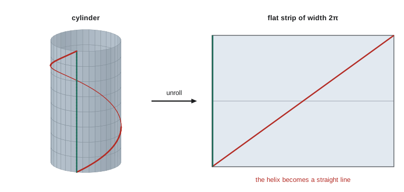
No perfect map. A piece of the sphere has \(K = 1/R^2\) and a piece of the plane has \(K = 0\), so no map between them preserves all lengths. Every map projection distorts something; lesson 6 showed that the distortions can be traded, conformal or equal-area, but not removed. The same argument shows that a cylinder or cone can be wrapped with paper without creasing or tearing, but a sphere cannot, as anyone who has wrapped a ball knows.

Bending surfaces. A sheet of paper can be bent into a cylinder or cone, but not into a saddle. A flat slice of pizza that droops can be stiffened by curling its crust: curling forces \(\kappa_1 \ne 0\) across the slice, and since bending preserves \(K = \kappa_1\kappa_2 = 0\), the other principal curvature along the slice must vanish, so the tip cannot droop. Corrugated roofing and the folded shells of some seashells exploit the same principle.

The helicoid and the catenoid. The helicoid \((v\cos u, v\sin u, u)\) has \(ds^2 = (1 + v^2)\,du^2 + dv^2\). Substitute \(v = \sinh w\): then \(dv = \cosh w\,dw\) and \(ds^2 = \cosh^2 w\,(du^2 + dw^2)\). The catenoid \((\cosh w\cos u, \cosh w\sin u, w)\) has exactly this first fundamental form (lesson 8). So the map sending the helicoid point with coordinates \((u, \sinh w)\) to the catenoid point with coordinates \((u, w)\) is a local isometry, wrapping each turn of the helicoid once around the catenoid. In fact the surfaces \(\cos t\) times the catenoid plus \(\sin t\) times its conjugate helicoid form a continuous family of minimal surfaces, all isometric, that bends one into the other.

Minding's theorem. Conversely, constant curvature is all there is locally: Ferdinand Minding proved in 1839 that any two surfaces with the same constant Gaussian curvature are locally isometric. Surfaces with \(K = -1\), such as the pseudosphere obtained by rotating a tractrix, were used by Eugenio Beltrami in 1868 to give the first concrete model of the non-Euclidean geometry of Lobachevsky and Bolyai. A theorem of David Hilbert from 1901 says that no complete surface of constant negative curvature can sit smoothly in \(\mathbb{R}^3\), which is why the pseudosphere has a sharp rim and abstract models like Poincaré's half-plane are needed.

The compatibility equations and Bonnet's theorem

The Theorema Egregium came from one consequence of \((\mathbf{x}_{uu})_v = (\mathbf{x}_{uv})_u\) and \((\mathbf{x}_{vv})_u = (\mathbf{x}_{uv})_v\). Expanding these identities fully in the frame and comparing components gives three equations: the Gauss equation, which is the Theorema Egregium, and the two Codazzi–Mainardi equations

found by Gaspare Mainardi in 1856 and Delfino Codazzi in 1860. They are necessary conditions on the six coefficients \(E, F, G, e, f, g\) for a surface to exist. Pierre Ossian Bonnet proved in 1867 that they are also sufficient.

Theorem (Bonnet). Let \(E, F, G, e, f, g\) be smooth functions on a simply connected open set \(U \subseteq \mathbb{R}^2\) with \(E > 0\) and \(EG - F^2 > 0\), satisfying the Gauss and Codazzi–Mainardi equations. Then there is a regular parametrized surface \(\mathbf{x} : U \to \mathbb{R}^3\) with these fundamental forms, unique up to a rigid motion.

The proof parallels the fundamental theorem of curves from lesson 3: the frame equations form a system of partial differential equations, the compatibility equations are exactly the integrability conditions guaranteeing that it has solutions (by the theorem of Frobenius), and uniqueness follows from the same kind of argument as for curves. The theorem says that the first fundamental form, which is intrinsic, and the second, which describes the bending, together determine the surface, just as curvature and torsion determine a curve.

Curvature from the metric alone

The program plays the role of the ant. It is given only the functions \(E, F, G\) of several metrics, never a map into space, and it computes \(K\) by Brioschi's formula with derivatives taken by finite differences. For the torus and the ellipsoid of revolution it compares the result with the extrinsic value \((eg - f^2)/(EG - F^2)\) computed from a parametrization in space. It also checks that the helicoid in the coordinates \((u, \sinh w)\) and the catenoid have identical coefficients and curvature, and evaluates two metrics with no surface behind them.

import math

def brioschi(E, F, G, u, v, h=1e-3):
    d = lambda f, du, dv: (f(u + du*h, v + dv*h) - f(u - du*h, v - dv*h)) / (2*h)
    d2 = lambda f, du, dv: (f(u + du*h, v + dv*h) - 2*f(u, v) + f(u - du*h, v - dv*h)) / h**2
    Fuv = (F(u + h, v + h) - F(u + h, v - h) - F(u - h, v + h) + F(u - h, v - h)) / (4*h*h)
    e_, f_, g_ = E(u, v), F(u, v), G(u, v)
    Eu, Ev, Fu, Fv, Gu, Gv = d(E, 1, 0), d(E, 0, 1), d(F, 1, 0), d(F, 0, 1), d(G, 1, 0), d(G, 0, 1)
    Evv, Guu = d2(E, 0, 1), d2(G, 1, 0)
    det3 = lambda m: (m[0][0]*(m[1][1]*m[2][2] - m[1][2]*m[2][1]) - m[0][1]*(m[1][0]*m[2][2] - m[1][2]*m[2][0])
                      + m[0][2]*(m[1][0]*m[2][1] - m[1][1]*m[2][0]))
    A = [[-Evv/2 + Fuv - Guu/2, Eu/2, Fu - Ev/2], [Fv - Gu/2, e_, f_], [Gv/2, f_, g_]]
    B = [[0, Ev/2, Gu/2], [Ev/2, e_, f_], [Gu/2, f_, g_]]
    return (det3(A) - det3(B)) / (e_*g_ - f_*f_)**2

R, r = 2.0, 1.0
metrics = {
    "unit sphere (lat, lon)":   (lambda u, v: 1.0, lambda u, v: 0.0, lambda u, v: math.cos(u)**2, (0.7, 0.2), 1.0),
    "torus R=2 r=1 (u, v)":     (lambda u, v: (R + r*math.cos(v))**2, lambda u, v: 0.0, lambda u, v: r*r, (0.3, 2.0),
                                 math.cos(2.0)/(r*(R + r*math.cos(2.0)))),
    "catenoid (u, w)":          (lambda u, w: math.cosh(w)**2, lambda u, w: 0.0, lambda u, w: math.cosh(w)**2, (0.4, 0.6),
                                 -1/math.cosh(0.6)**4),
    "helicoid (u, v = sinh w)": (lambda u, w: 1 + math.sinh(w)**2, lambda u, w: 0.0, lambda u, w: math.cosh(w)**2, (0.4, 0.6),
                                 -1/(1 + math.sinh(0.6)**2)**2),
    "graph z = x^2 + y^2":      (lambda x, y: 1 + 4*x*x, lambda x, y: 4*x*y, lambda x, y: 1 + 4*y*y, (0.5, -0.3),
                                 4/(1 + 4*0.25 + 4*0.09)**2),
    "Poincare half-plane":      (lambda x, y: 1/y**2, lambda x, y: 0.0, lambda x, y: 1/y**2, (0.3, 1.7), -1.0),
    "du^2 + e^(2u) dv^2":       (lambda u, v: 1.0, lambda u, v: 0.0, lambda u, v: math.exp(2*u), (0.4, 0.0), -1.0),
}
for name, (E, F, G, (u, v), exact) in metrics.items():
    print(f"{name:26s} K from metric = {brioschi(E, F, G, u, v):+.6f}   expected {exact:+.6f}")

# extrinsic check for an ellipsoid of revolution x = (2 cos v cos u, 2 cos v sin u, sin v)
def X(u, v): return [2*math.cos(v)*math.cos(u), 2*math.cos(v)*math.sin(u), math.sin(v)]
def partial(f, u, v, i, h=1e-4):
    a = f(u + h, v) if i == 0 else f(u, v + h); b = f(u - h, v) if i == 0 else f(u, v - h)
    return [(p - q)/(2*h) for p, q in zip(a, b)]
dot = lambda a, b: sum(x*y for x, y in zip(a, b))
Ef = lambda u, v: dot(partial(X, u, v, 0), partial(X, u, v, 0))
Ff = lambda u, v: dot(partial(X, u, v, 0), partial(X, u, v, 1))
Gf = lambda u, v: dot(partial(X, u, v, 1), partial(X, u, v, 1))
u, v = 0.5, 0.8
exact = 1 / (4 * (math.sin(v)**2 + math.cos(v)**2 / 4)**2) / 4   # 1/(a^2 c^2 (x^2/a^4 + y^2/b^4 + z^2/c^4)^2) for a = b = 2, c = 1
print(f"ellipsoid of revolution: K intrinsic = {brioschi(Ef, Ff, Gf, u, v, 1e-3):+.5f}   extrinsic formula {exact:+.5f}")

unit sphere (lat, lon)     K from metric = +0.999999   expected +1.000000
torus R=2 r=1 (u, v)       K from metric = -0.262743   expected -0.262743
catenoid (u, w)            K from metric = -0.506343   expected -0.506343
helicoid (u, v = sinh w)   K from metric = -0.506343   expected -0.506343
graph z = x^2 + y^2        K from metric = +0.718184   expected +0.718184
Poincare half-plane        K from metric = -0.999999   expected -1.000000
du^2 + e^(2u) dv^2         K from metric = -0.999999   expected -1.000000
ellipsoid of revolution: K intrinsic = +0.15454   extrinsic formula +0.15454

Every value agrees with the expected one to about six digits, the error coming from finite differences with step \(10^{-3}\). The sphere, torus, catenoid and paraboloid values match the extrinsic formulas of lesson 8 although the program never sees a normal vector. The helicoid in the coordinates \((u, \sinh w)\) and the catenoid have identical metrics and therefore identical curvature, \(-1/\cosh^4(0.6) \approx -0.5063\), at corresponding points. The Poincaré half-plane and the metric \(du^2 + e^{2u}\,dv^2\) are not given by any surface in space, yet the formula still assigns them curvature \(-1\): the ant's geometry makes sense without a surrounding space, an idea lesson 12 develops. The last line computes \(K\) for an ellipsoid of revolution from \(E, F, G\) obtained by differentiating the embedding, and it matches the classical extrinsic formula.