Gaussian and mean curvature, principal curvatures and minimal surfaces

The shape operator of lesson 7 is a self-adjoint map of each tangent plane, so linear algebra hands us its eigenvalues and eigenvectors. The eigenvalues, the principal curvatures, are the largest and smallest normal curvatures at the point, and the directions in which they occur are perpendicular. Their product is the Gaussian curvature \(K\) and their average the mean curvature \(H\). This lesson computes these invariants, classifies points by the sign of \(K\), characterizes spheres as the surfaces that curve equally in all directions, proves that a closed surface must somewhere be curved like a sphere, and introduces minimal surfaces, those with \(H = 0\), which are the critical points of area.

Principal curvatures and Euler's formula

Let \(S_p = -dN_p\) be the shape operator at \(p\). By the spectral theorem there is an orthonormal basis \(e_1, e_2\) of \(T_pS\) with \(S_p e_1 = \kappa_1 e_1\) and \(S_p e_2 = \kappa_2 e_2\), where we order \(\kappa_1 \ge \kappa_2\). These are the principal curvatures, and \(e_1, e_2\) the principal directions. A unit tangent vector making angle \(\theta\) with \(e_1\) is \(w = \cos\theta\,e_1 + \sin\theta\,e_2\), and its normal curvature is

This is Euler's formula of 1760. It shows that \(\kappa_1\) and \(\kappa_2\) are the maximum and minimum of the normal curvature over all directions, and that the normal curvature in any direction is a weighted average of the two. If \(\kappa_1 = \kappa_2\), every direction is principal and the point is called umbilic; spheres and planes consist entirely of umbilic points.

Gaussian and mean curvature

The Gaussian curvature and the mean curvature are

Using the matrix \(A = I^{-1}II\) of the Weingarten equations, the determinant and trace give formulas in any patch:

The principal curvatures are then the roots of \(\kappa^2 - 2H\kappa + K = 0\), namely \(\kappa = H \pm \sqrt{H^2 - K}\); the discriminant \(H^2 - K = \frac14(\kappa_1 - \kappa_2)^2\) is nonnegative and vanishes exactly at umbilics. Reversing the normal changes the signs of \(\kappa_1, \kappa_2\) and \(H\) but leaves \(K\) unchanged. So \(K\) is defined even on non-orientable surfaces, while \(H\) needs an orientation.

Examples. A sphere of radius \(R\) with inward normal has \(\kappa_1 = \kappa_2 = 1/R\), so \(K = 1/R^2\) and \(H = 1/R\). A cylinder of radius \(R\) has \(\kappa_1 = 1/R\) around the circle and \(\kappa_2 = 0\) along the rulings, so \(K = 0\) and \(H = 1/(2R)\). The saddle \(z = xy\) at the origin has \(e = g = 0\), \(f = 1\), \(E = G = 1\), \(F = 0\), so \(K = -1\), \(H = 0\), with principal curvatures \(\pm 1\) in the diagonal directions \(y = \pm x\). The torus with outward normal has, from lesson 7, \(\kappa\) along parallels equal to \(-\cos v/(R + r\cos v)\) and along meridians \(-1/r\), so \(K = \frac{\cos v}{r(R + r\cos v)}\).

Classifying points

The sign of \(K\) describes the shape of the surface near \(p\), via the height function of lesson 7. Choose coordinates with \(p\) at the origin, \(T_pS\) the \(xy\)-plane and the axes along the principal directions. Then the surface is locally a graph

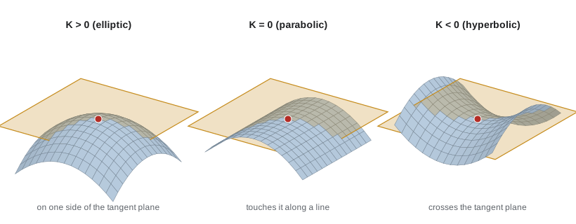
A point is elliptic if \(K > 0\): the principal curvatures have the same sign, the quadratic part is definite and the surface lies locally on one side of its tangent plane, like a sphere or the outside of a torus. It is hyperbolic if \(K < 0\): the quadratic part is indefinite and the surface crosses its tangent plane in a saddle, like the inside of a torus. It is parabolic if \(K = 0\) but \(S_p \ne 0\), like every point of a cylinder, and planar if \(S_p = 0\), like every point of a plane or the origin of the monkey saddle \(z = x^3 - 3xy^2\). At a hyperbolic point the directions with \(\kappa_n = 0\), the asymptotic directions, satisfy \(\tan^2\theta = -\kappa_1/\kappa_2\), and they bisect the principal directions exactly when \(H = 0\).

Surfaces made of umbilics

Theorem. If every point of a connected regular surface \(S\) is umbilic, then \(S\) is contained in a plane or a sphere.

Proof. At each point \(dN = -\lambda\,\mathrm{id}\) for some number \(\lambda(p)\). In a connected patch, \(N_u = -\lambda\mathbf{x}_u\) and \(N_v = -\lambda\mathbf{x}_v\). Differentiate the first with respect to \(v\) and the second with respect to \(u\) and subtract: \(0 = N_{uv} - N_{vu} = -\lambda_v\mathbf{x}_u + \lambda_u\mathbf{x}_v\). Since \(\mathbf{x}_u, \mathbf{x}_v\) are independent, \(\lambda_u = \lambda_v = 0\), so \(\lambda\) is constant on the patch, and by connectedness on all of \(S\) (the set where \(\lambda\) takes a given value is open and closed). If \(\lambda = 0\), \(N\) is constant and \(S\) lies in a plane (lesson 7, practice problem 4). If \(\lambda \ne 0\), consider \(\mathbf{x} + \frac{1}{\lambda}N\): its derivatives are \(\mathbf{x}_u + \frac{1}{\lambda}N_u = 0\) and likewise for \(v\), so it is a constant point \(c\). Then \(|\mathbf{x} - c| = 1/|\lambda|\) and \(S\) lies on the sphere of that radius about \(c\). \(\blacksquare\)

Compact surfaces have elliptic points

Theorem. Every compact regular surface in \(\mathbb{R}^3\) has a point where \(K > 0\).

Proof. The continuous function \(|x|^2\) attains its maximum on the compact surface at some point \(p\); let \(\rho = |p| > 0\). The surface lies inside the closed ball of radius \(\rho\), touching the sphere of radius \(\rho\) at \(p\). The tangent plane at \(p\) is perpendicular to \(p\), since \(p\) maximizes \(|x|^2\) and so the derivative \(2\langle p, w \rangle\) vanishes for tangent \(w\). Take \(N(p) = -p/\rho\), pointing inward. For any unit-speed curve \(\alpha\) on \(S\) with \(\alpha(0) = p\), the function \(|\alpha(s)|^2\) has a maximum at \(s = 0\), so its second derivative \(2|\alpha'|^2 + 2\langle \alpha, \alpha'' \rangle = 2 + 2\langle p, \alpha''(0) \rangle\) is at most zero. Hence the normal curvature \(\kappa_n = \langle \alpha'', N \rangle = -\langle \alpha'', p \rangle/\rho \ge 1/\rho\). Every normal curvature at \(p\) is at least \(1/\rho\), so \(\kappa_1, \kappa_2 \ge 1/\rho\) and \(K \ge 1/\rho^2 > 0\). \(\blacksquare\)

A consequence: there is no compact surface in \(\mathbb{R}^3\) with \(K \le 0\) everywhere. In particular no compact minimal surface exists, since \(H = 0\) forces \(K = -\kappa_1^2 \le 0\). The torus, which is compact, has positive curvature on its outer half. Heinrich Liebmann proved in 1899 the stronger statement that a compact connected surface with constant Gaussian curvature is a round sphere, and Heinz Hopf in 1951 and Aleksandr Aleksandrov in 1956 proved the corresponding rigidity theorems for constant mean curvature.

Minimal surfaces

A surface is minimal if \(H = 0\) at every point, so that its principal curvatures are opposite, \(\kappa_2 = -\kappa_1\). The name comes from the following fact, which explains why soap films, which minimize area to minimize surface energy, are minimal surfaces.

Theorem. Let \(\mathbf{x} : U \to S\) be a patch, \(Q \subset U\) a compact region with smooth boundary, and \(\phi\) a smooth function on \(U\) vanishing outside a compact subset of the interior of \(Q\). For the normal variation \(\mathbf{x}^t = \mathbf{x} + t\phi N\), the area \(A(t)\) of \(\mathbf{x}^t(Q)\) satisfies

Proof. Compute \(\mathbf{x}^t_u = \mathbf{x}_u + t\phi N_u + t\phi_u N\) and similarly for \(v\). Then \(E^t = E + 2t\phi\langle \mathbf{x}_u, N_u \rangle + O(t^2) = E - 2t\phi e + O(t^2)\), using \(\langle \mathbf{x}_u, N \rangle = 0\); likewise \(F^t = F - 2t\phi f + O(t^2)\) and \(G^t = G - 2t\phi g + O(t^2)\). Therefore \(E^tG^t - (F^t)^2 = EG - F^2 - 2t\phi(eG - 2fF + gE) + O(t^2) = (EG - F^2)(1 - 4t\phi H) + O(t^2)\). Taking square roots, \(\sqrt{E^tG^t - (F^t)^2} = \sqrt{EG - F^2}\,(1 - 2t\phi H) + O(t^2)\), and differentiating the area integral at \(t = 0\) gives the formula. \(\blacksquare\)

So \(A'(0) = 0\) for every variation if and only if \(H \equiv 0\): minimal surfaces are exactly the critical points of area. (They need not be minimizers, just as a critical point of a function need not be a minimum.) The vector \(2HN\), the mean curvature vector, points in the direction in which area decreases fastest, which is why a soap bubble with different pressures on its two sides has constant nonzero mean curvature: the Young–Laplace law says the pressure jump is \(2\sigma H\), with \(\sigma\) the surface tension.

The catenoid and the helicoid

The first nonplanar minimal surface was found by Euler in 1744: the catenoid, obtained by rotating the catenary \(x = \cosh z\) about the \(z\)-axis, parametrized by \(\mathbf{x}(u, v) = (\cosh v\cos u, \cosh v\sin u, v)\). From lesson 7 with profile \(f = \cosh v\), \(g = v\): \(E = \cosh^2 v\), \(F = 0\), \(G = \sinh^2 v + 1 = \cosh^2 v\), and the normal \(N = \frac{1}{\cosh v}(\cos u, \sin u, -\sinh v)\) gives \(e = -1\), \(f = 0\), \(g = 1\). So

The catenoid is minimal, with curvature most negative on its waist. It is the shape of a soap film stretched between two coaxial rings close enough together; when the rings are pulled apart beyond about 1.325 times their radius, the catenoid becomes unstable and the film snaps into two flat discs. Meusnier found the second example in 1776, the helicoid \(\mathbf{x}(u, v) = (v\cos u, v\sin u, u)\), swept out by a horizontal line rising and rotating uniformly, the shape of a spiral staircase or an Archimedean screw. With \(E = 1 + v^2\), \(F = 0\), \(G = 1\) from lesson 6, the normal \(N = \frac{1}{\sqrt{1 + v^2}}(\sin u, -\cos u, v)\) and \(\mathbf{x}_{uu} = (-v\cos u, -v\sin u, 0)\), \(\mathbf{x}_{uv} = (-\sin u, \cos u, 0)\), \(\mathbf{x}_{vv} = 0\) give \(e = 0\), \(f = -1/\sqrt{1 + v^2}\), \(g = 0\), so \(H = 0\) and \(K = -1/(1 + v^2)^2\).

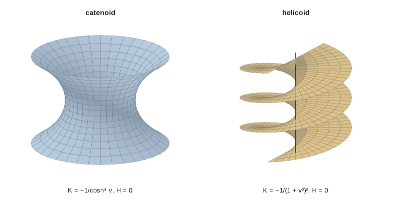
The catenoid and helicoid have the same Gaussian curvature at corresponding points under the substitution \(v = \sinh w\) on the helicoid, and lesson 9 shows that they are in fact locally isometric: a piece of helicoid can be bent into a piece of catenoid without stretching, through a family of minimal surfaces. Plateau's problem, posed by Lagrange in 1760 and named for the Belgian physicist Joseph Plateau, who experimented with soap films in the 1840s, asks whether every closed curve in space bounds a minimal surface. Jesse Douglas and Tibor Radó solved it independently around 1930, and Douglas received one of the first two Fields Medals in 1936. New complete embedded minimal surfaces were found by Heinrich Scherk in 1834 and, after a long gap, by Celso Costa in 1982.

Computing curvatures

The program computes \(K\), \(H\) and the principal curvatures numerically from \(E, F, G, e, f, g\) for the ellipsoid, catenoid, helicoid and monkey saddle, compares with exact values, verifies Euler's formula by sampling normal curvatures in many directions, and checks the first variation formula on the catenoid by computing the area of a slightly pushed surface.

import math

def dot(a, b): return sum(x*y for x, y in zip(a, b))
def cross(a, b): return [a[1]*b[2] - a[2]*b[1], a[2]*b[0] - a[0]*b[2], a[0]*b[1] - a[1]*b[0]]
def unit(a):
    n = math.sqrt(dot(a, a)); return [x/n for x in a]
def forms(X, u, v, h=1e-4):
    P = lambda i, j: X(u + i*h, v + j*h)
    xu = [(a - b)/(2*h) for a, b in zip(P(1, 0), P(-1, 0))]
    xv = [(a - b)/(2*h) for a, b in zip(P(0, 1), P(0, -1))]
    xuu = [(a - 2*m + b)/h**2 for a, m, b in zip(P(1, 0), P(0, 0), P(-1, 0))]
    xvv = [(a - 2*m + b)/h**2 for a, m, b in zip(P(0, 1), P(0, 0), P(0, -1))]
    xuv = [(a - b - c + d)/(4*h*h) for a, b, c, d in zip(P(1, 1), P(1, -1), P(-1, 1), P(-1, -1))]
    N = unit(cross(xu, xv))
    return dot(xu, xu), dot(xu, xv), dot(xv, xv), dot(N, xuu), dot(N, xuv), dot(N, xvv), xu, xv
def curv(X, u, v):
    E, F, G, e, f, g, xu, xv = forms(X, u, v)
    K = (e*g - f*f)/(E*G - F*F); H = (e*G - 2*f*F + g*E)/(2*(E*G - F*F))
    d = math.sqrt(max(H*H - K, 0))
    return K, H, H + d, H - d

surfaces = {
    "ellipsoid 2,1,0.5": (lambda u, v: [2*math.cos(v)*math.cos(u), math.cos(v)*math.sin(u), 0.5*math.sin(v)], 0.0, 0.0),
    "catenoid":          (lambda u, v: [math.cosh(v)*math.cos(u), math.cosh(v)*math.sin(u), v], 0.3, 0.5),
    "helicoid":          (lambda u, v: [v*math.cos(u), v*math.sin(u), u], 0.3, 0.5),
    "monkey saddle":     (lambda u, v: [u, v, u**3 - 3*u*v*v], 0.0, 0.0),
}
for name, (X, u, v) in surfaces.items():
    K, H, k1, k2 = curv(X, u, v)
    print(f"{name:18s} at ({u},{v}): K={K:+.6f}  H={H:+.6f}  k1={k1:+.6f}  k2={k2:+.6f}")
print("exact: ellipsoid at (2, 0, 0) has |k1|, |k2| = a/c^2 = 8, a/b^2 = 2 and K = 16")
print(f"exact: catenoid K = -1/cosh^4(0.5) = {-1/math.cosh(0.5)**4:+.6f}; helicoid K = -1/(1+0.25)^2 = {-1/1.25**2:+.6f}")

# Euler's formula on the ellipsoid at a general point
X = surfaces["ellipsoid 2,1,0.5"][0]
u, v = 0.6, 0.4
E, F, G, e, f, g, xu, xv = forms(X, u, v)
K, H, k1, k2 = curv(X, u, v)
kns = []
for k in range(360):
    t = math.radians(k * 0.5)
    a, b = math.cos(t), math.sin(t)
    kns.append((e*a*a + 2*f*a*b + g*b*b) / (E*a*a + 2*F*a*b + G*b*b))
print(f"normal curvatures over 180 directions: max {max(kns):+.6f} min {min(kns):+.6f}  vs k1 {k1:+.6f} k2 {k2:+.6f}")

# first variation on the catenoid: push by t*phi*N, phi = bump in v, compare dA/dt with -2 int phi H dA = 0
cat = surfaces["catenoid"][0]
def area_pushed(t, n=120):
    A = 0.0
    for i in range(n):
        for j in range(n):
            u = 2*math.pi*(i + 0.5)/n; v = -1 + 2*(j + 0.5)/n
            def Y(uu, vv):
                phi = math.cos(math.pi*vv/2)**2           # vanishes at the boundary v = -1, 1
                E, F, G, e, f, g, a, b = forms(cat, uu, vv, 1e-5)
                N = unit(cross(a, b))
                return [p + t*phi*q for p, q in zip(cat(uu, vv), N)]
            E, F, G, *_ = forms(Y, u, v, 1e-4)
            A += math.sqrt(E*G - F*F) * (2*math.pi/n) * (2/n)
    return A
A0, Ap, Am = area_pushed(0.0, 40), area_pushed(0.01, 40), area_pushed(-0.01, 40)
print(f"catenoid area {A0:.6f}; (A(0.01) - A(-0.01))/0.02 = {(Ap - Am)/0.02:+.2e}; second difference {(Ap - 2*A0 + Am)/1e-4:+.4f}")

ellipsoid 2,1,0.5  at (0.0,0.0): K=+16.000000  H=-5.000000  k1=-2.000000  k2=-8.000000
catenoid           at (0.3,0.5): K=-0.618500  H=+0.000000  k1=+0.786448  k2=-0.786448
helicoid           at (0.3,0.5): K=-0.640000  H=+0.000000  k1=+0.800000  k2=-0.800000
monkey saddle      at (0.0,0.0): K=+0.000000  H=+0.000000  k1=+0.000000  k2=+0.000000
exact: ellipsoid at (2, 0, 0) has |k1|, |k2| = a/c^2 = 8, a/b^2 = 2 and K = 16
exact: catenoid K = -1/cosh^4(0.5) = -0.618500; helicoid K = -1/(1+0.25)^2 = -0.640000
normal curvatures over 180 directions: max -0.458834 min -2.088446  vs k1 -0.458830 k2 -2.088556
catenoid area 17.672557; (A(0.01) - A(-0.01))/0.02 = +6.50e-04; second difference +6.7428

With the normal \(\mathbf{x}_u \times \mathbf{x}_v\), which points outward on this ellipsoid, the principal curvatures at \((2, 0, 0)\) are \(-2\) and \(-8\), magnitudes \(a/b^2\) and \(a/c^2\): the surface is most sharply curved in the direction of its shortest axis. Their product \(K = 16\) and average \(H = -5\) follow. The catenoid and helicoid have \(H = 0\) to six digits and principal curvatures of opposite sign, with \(K\) matching the exact formulas; the monkey saddle has a planar point at the origin. Sampling the normal curvature over half a turn of directions recovers \(\kappa_1\) and \(\kappa_2\) as its maximum and minimum, which is Euler's formula. Finally, pushing a band of the catenoid along its normal changes the area at first order by an amount indistinguishable from zero (the residue \(6.5 \times 10^{-4}\) comes from the coarse 40 by 40 grid), while the second difference is positive: this short band of catenoid is a local minimum of area, not merely a critical point.