
MATH-430 · Lesson 10 of 12 · 28 min
Geodesics and the covariant derivative
What is a straight line on a curved surface? A line in the plane can be characterized in several ways: its tangent never turns, it has zero acceleration, and it is locally the shortest path between its points. On a surface we cannot ask for zero acceleration in space, since a curve on a sphere must accelerate toward the center just to stay on the sphere. The right notion is that the acceleration has no component within the surface: the curve does not turn as seen by an inhabitant. This lesson defines the covariant derivative, the derivative of vector fields as the ant measures it, and uses it to define parallel transport and geodesics. Both turn out to be intrinsic, computable from \(E\), \(F\), \(G\) through the Christoffel symbols of lesson 9.
The covariant derivative
Let \(\alpha(t)\) be a curve on an oriented surface \(S\) and \(w(t)\) a smooth vector field along it, with \(w(t) \in T_{\alpha(t)}S\) for each \(t\). The ordinary derivative \(w'(t)\) is a vector in \(\mathbb{R}^3\) that usually sticks out of the tangent plane. The covariant derivative is its tangential part,
the orthogonal projection of \(w'\) onto \(T_{\alpha(t)}S\). It is the rate of change of \(w\) that an observer confined to the surface can perceive. It obeys the product rules \(\frac{D}{dt}(fw) = f'w + f\frac{Dw}{dt}\) and \(\frac{d}{dt}\langle w_1, w_2 \rangle = \langle \frac{Dw_1}{dt}, w_2 \rangle + \langle w_1, \frac{Dw_2}{dt} \rangle\); the second holds because the normal parts of \(w_1'\) and \(w_2'\) are orthogonal to the tangent vectors \(w_2\) and \(w_1\).
Theorem. The covariant derivative is intrinsic. If \(\alpha(t) = \mathbf{x}(u(t), v(t))\) and \(w = a(t)\mathbf{x}_u + b(t)\mathbf{x}_v\), then
Proof. Differentiate: \(w' = a'\mathbf{x}_u + b'\mathbf{x}_v + a(\mathbf{x}_{uu}u' + \mathbf{x}_{uv}v') + b(\mathbf{x}_{vu}u' + \mathbf{x}_{vv}v')\). Substitute the expansions of \(\mathbf{x}_{uu}, \mathbf{x}_{uv}, \mathbf{x}_{vv}\) from lesson 9 and discard the multiples of \(N\). Collecting the coefficients of \(\mathbf{x}_u\) and \(\mathbf{x}_v\) gives the formula. Since the Christoffel symbols depend only on the first fundamental form, so does \(Dw/dt\). \(\blacksquare\)
The formula uses only the curve's coordinates, the vector's components and the Christoffel symbols. In the plane with Cartesian coordinates all symbols vanish and the covariant derivative is the ordinary derivative. In polar coordinates it is not: the unit vector \(\mathbf{x}_r\) along a circle \(r = 1\), \(\theta = t\) has \(a = 1\), \(b = 0\), \(u' = 0\), \(v' = 1\), and \(D\mathbf{x}_r/dt = \Gamma^2_{12}\mathbf{x}_\theta = \mathbf{x}_\theta\), a reminder that radial unit vectors rotate as we go around.
Parallel transport
A vector field \(w\) along \(\alpha\) is parallel if \(Dw/dt = 0\). In coordinates this is a linear system of two first-order differential equations for \(a(t), b(t)\), so for any initial vector \(w_0 \in T_{\alpha(t_0)}S\) there is a unique parallel field along \(\alpha\) with \(w(t_0) = w_0\). Its value at a later time \(t_1\) is the parallel transport of \(w_0\) along \(\alpha\), written \(P_{\alpha}(w_0) \in T_{\alpha(t_1)}S\).
Theorem. Parallel transport is a linear isometry: it preserves lengths of vectors and angles between them.
Proof. Linearity follows from linearity of the equations. If \(w_1\) and \(w_2\) are parallel, the product rule gives \(\frac{d}{dt}\langle w_1, w_2 \rangle = \langle \frac{Dw_1}{dt}, w_2 \rangle + \langle w_1, \frac{Dw_2}{dt} \rangle = 0\), so their inner product is constant. \(\blacksquare\)
On a plane, parallel transport is ordinary translation of vectors, independent of the path. On a curved surface it depends on the path. Picture carrying a spear around the triangle of lesson 1 on the sphere, always keeping it parallel: start at the north pole pointing south along one meridian, walk down to the equator keeping the spear pointing straight ahead, walk a quarter of the way around the equator with the spear pointing perpendicular to your path, and walk back up. At the pole the spear has turned through a right angle, equal to the area of the triangle. The rotation of vectors transported around a closed loop is the holonomy of the loop, and lesson 11 proves that on any surface it equals the integral of \(K\) over the enclosed region.
Worked problem
Holonomy around a circle of latitude
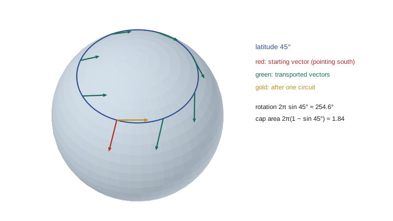
On the unit sphere with \(ds^2 = d\varphi^2 + \cos^2\varphi\,d\theta^2\), transport a vector parallel around the latitude circle \(\varphi = \varphi_0\), \(\theta = t\), \(0 \le t \le 2\pi\). By how much is it rotated?
Show solution
- From lesson 9, the nonzero symbols are \(\Gamma^2_{12} = -\tan\varphi\) and \(\Gamma^1_{22} = \sin\varphi\cos\varphi\). Along the curve \(u' = \varphi' = 0\), \(v' = \theta' = 1\).
- The parallel transport equations are \(a' + \Gamma^1_{22}b = 0\) and \(b' + \Gamma^2_{12}a = 0\), that is \(a' = -\sin\varphi_0\cos\varphi_0\,b\) and \(b' = \tan\varphi_0\,a\).
- Use orthonormal components \(A = a\) along \(\mathbf{x}_\varphi\) and \(B = \cos\varphi_0\,b\) along the unit vector \(\mathbf{x}_\theta/\cos\varphi_0\). Then \(A' = -\sin\varphi_0\,B\) and \(B' = \sin\varphi_0\,A\).
- This is uniform rotation at rate \(\sin\varphi_0\): \((A, B)\) turns by the angle \(\sin\varphi_0\,t\) relative to the orthonormal frame, counterclockwise.
- The northward and eastward unit vectors form a frame that returns to itself after one circuit, \(t = 2\pi\), so relative to its starting position the transported vector has rotated by \(2\pi\sin\varphi_0\). Since \(2\pi\sin\varphi_0 = 2\pi - 2\pi(1 - \sin\varphi_0)\), this is the same as a rotation by \(-2\pi(1 - \sin\varphi_0)\).
Answer: The vector returns rotated by \(2\pi\sin\varphi_0\), equivalently by \(-2\pi(1 - \sin\varphi_0)\) modulo \(2\pi\). The number \(2\pi(1 - \sin\varphi_0)\) is the area of the polar cap above the circle. On the equator \(\varphi_0 = 0\) there is no rotation, because the equator is a geodesic, and near the pole the cap is small and the rotation is nearly a full turn, indistinguishable from none.
Foucault's pendulum illustrates this. Its plane of swing is carried by the rotating Earth around a circle of latitude in one sidereal day, and relative to the ground it precesses by \(2\pi\sin\varphi_0\) per day: once a day at the poles, not at all on the equator, and about 271 degrees a day at the latitude of Paris, where Léon Foucault demonstrated it in 1851. The pendulum is parallel transporting its plane of swing.
Geodesics
A curve \(\gamma\) on \(S\) is a geodesic if its velocity is parallel along it, \(\frac{D\gamma'}{dt} = 0\). Equivalently, its acceleration \(\gamma''\) is everywhere normal to the surface. Since \(\frac{d}{dt}|\gamma'|^2 = 2\langle \frac{D\gamma'}{dt}, \gamma' \rangle = 0\), geodesics have constant speed. Writing \(\gamma(t) = \mathbf{x}(u(t), v(t))\) and applying the coordinate formula to \(w = \gamma' = u'\mathbf{x}_u + v'\mathbf{x}_v\) gives the geodesic equations
These are second-order ordinary differential equations with smooth coefficients, so through every point \(p\) and in every direction \(w \in T_pS\) there is a unique geodesic \(\gamma_w\) with \(\gamma_w(0) = p\) and \(\gamma_w'(0) = w\), defined for \(t\) in some interval around 0. Geodesics are intrinsic: local isometries carry geodesics to geodesics.
Examples. On a plane the Christoffel symbols vanish in Cartesian coordinates and geodesics are straight lines traversed at constant speed. On a sphere, great circles traversed at constant speed are geodesics, since their acceleration points to the center, which is normal to the sphere; by uniqueness these are all the geodesics. On a cylinder, unrolling is a local isometry to the plane, so geodesics are the images of lines: rulings, horizontal circles and helices, as the figure in lesson 9 showed. Through two points on a cylinder there are infinitely many geodesics, winding around different numbers of times.
Geodesic curvature
For a unit-speed curve \(\alpha\) on an oriented surface, the vectors \(\alpha'\), \(N \times \alpha'\) and \(N\) form an orthonormal frame, the Darboux frame. Since \(\alpha'' \perp \alpha'\), the acceleration splits as
The normal curvature \(\kappa_n = II(\alpha')\) is what Meusnier's theorem described. The geodesic curvature \(\kappa_g = \langle \frac{D\alpha'}{ds}, N \times \alpha' \rangle\) measures how much the curve turns within the surface, and it is intrinsic, up to sign. Geodesics are exactly the curves with \(\kappa_g = 0\). A circle of latitude \(\varphi_0\) on the unit sphere has \(\kappa = 1/\cos\varphi_0\) and \(\kappa_n = 1\), so \(\kappa_g = \tan\varphi_0\): the latitude circles turn toward the pole, by an amount that vanishes only on the equator.
Clairaut's relation
On a surface of revolution with \(ds^2 = f(v)^2\,du^2 + dv^2\), the geodesic equations can be integrated once by a conservation law.
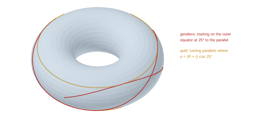
Theorem (Clairaut, 1733). Let \(\gamma\) be a unit-speed geodesic on a surface of revolution, let \(\rho = f(v)\) be the distance from the axis, and let \(\psi\) be the angle between \(\gamma'\) and the parallel through the point. Then \(\rho\cos\psi\) is constant along \(\gamma\).
Proof. Here \(E = f^2\), \(F = 0\), \(G = 1\), so \(\Gamma^1_{11} = 0\), \(\Gamma^1_{12} = f'/f\), \(\Gamma^1_{22} = 0\). The first geodesic equation reads \(u'' + 2\frac{f'}{f}u'v' = 0\), that is \(\frac{d}{ds}\big(f^2u'\big) = f^2u'' + 2ff'v'u' = 0\). So \(f^2u'\) is constant. The unit vector along the parallel is \(\mathbf{x}_u/f\), so \(\cos\psi = \langle \gamma', \mathbf{x}_u/f \rangle = f^2u'/f = fu'\), and \(\rho\cos\psi = f^2u'\). \(\blacksquare\)
Clairaut's relation is the conservation of angular momentum about the axis for a particle sliding freely on the surface. It explains the behavior of geodesics on a torus or a vase: a geodesic leaving a wide parallel at angle \(\psi_0\) can only reach parallels with \(\rho \ge \rho_0\cos\psi_0\), so geodesics that start nearly along a parallel are trapped in the wide outer region, oscillating between two parallels, while steeper ones pass through the hole.
Geodesics as critical points of length
Why are geodesics the straightest and, locally, the shortest curves? Consider the energy of a curve, \(\mathcal{E}(\alpha) = \frac12\int_a^b |\alpha'|^2\,dt = \frac12\int_a^b (Eu'^2 + 2Fu'v' + Gv'^2)\,dt\). For a variation \(\alpha_\varepsilon\) with fixed endpoints and variation field \(V = \partial\alpha_\varepsilon/\partial\varepsilon\) at \(\varepsilon = 0\), differentiating under the integral and integrating by parts gives the first variation formula
where the first step uses that mixed partial derivatives of the variation commute after projection, \(\frac{D}{d\varepsilon}\frac{\partial\alpha}{\partial t} = \frac{D}{dt}\frac{\partial\alpha}{\partial\varepsilon}\), and the boundary term vanishes because \(V = 0\) at the endpoints. The energy is stationary for all variations exactly when \(D\alpha'/dt = 0\): geodesics are the critical points of energy, and, since constant-speed reparametrization relates energy and length by the Cauchy–Schwarz inequality \(L^2 \le 2(b - a)\mathcal{E}\), they are critical points of length too. One can show, using geodesic polar coordinates, that a geodesic is the shortest curve between any two of its points that are close enough. Globally this can fail: an arc of a great circle longer than half the circle is a geodesic but not the shortest path between its endpoints.
The second variation brings in curvature. If \(\gamma\) is a unit-speed geodesic and \(J(s)\) measures the distance from \(\gamma\) to a nearby geodesic in the normal direction, then to first order \(J'' + K(\gamma(s))\,J = 0\), the Jacobi equation. Where \(K > 0\) nearby geodesics oscillate and reconverge, as meridians from the north pole meet again at the south pole; where \(K \le 0\) they spread apart and never meet again. This is the precise form of the remark in lesson 9 about \(\sqrt{G}\).
Integrating the geodesic equations
The program integrates the geodesic equations with the fourth-order Runge–Kutta method, using Christoffel symbols computed from the metric. On the unit sphere it starts a geodesic at latitude 20 degrees heading northeast and checks that it stays on a great circle by testing that its points lie in a plane through the origin. On the torus with \(R = 2\), \(r = 1\) it checks Clairaut's relation and reports the range of latitudes the geodesic visits. Finally it solves the parallel transport equations around several circles of latitude and compares the rotation with \(2\pi\sin\varphi_0\).
import math

def christoffel(E, G, Eu, Ev, Gu, Gv):
    """Christoffel symbols for an orthogonal metric (F = 0)."""
    return {(1, 11): Eu/(2*E), (2, 11): -Ev/(2*G), (1, 12): Ev/(2*E), (2, 12): Gu/(2*G), (1, 22): -Gu/(2*E), (2, 22): Gv/(2*G)}

def rk4(f, y, h, n):
    out = [y]
    for _ in range(n):
        k1 = f(y); k2 = f([a + h/2*b for a, b in zip(y, k1)]); k3 = f([a + h/2*b for a, b in zip(y, k2)]); k4 = f([a + h*b for a, b in zip(y, k3)])
        y = [a + h/6*(b + 2*c + 2*d + e) for a, b, c, d, e in zip(y, k1, k2, k3, k4)]
        out.append(y)
    return out

def geodesic_rhs(metric):
    def f(y):
        u, v, du, dv = y
        G_ = christoffel(*metric(u, v))
        ddu = -(G_[(1, 11)]*du*du + 2*G_[(1, 12)]*du*dv + G_[(1, 22)]*dv*dv)
        ddv = -(G_[(2, 11)]*du*du + 2*G_[(2, 12)]*du*dv + G_[(2, 22)]*dv*dv)
        return [du, dv, ddu, ddv]
    return f

# unit sphere, u = latitude, v = longitude: E = 1, G = cos^2 u
sphere = lambda u, v: (1.0, math.cos(u)**2, 0.0, 0.0, -2*math.sin(u)*math.cos(u), 0.0)
u0 = math.radians(20); a = math.radians(45)          # heading 45 degrees east of north
y0 = [u0, 0.0, math.cos(a), math.sin(a)/math.cos(u0)]  # unit speed
path = rk4(geodesic_rhs(sphere), y0, 0.01, 628)
P = [[math.cos(u)*math.cos(v), math.cos(u)*math.sin(v), math.sin(u)] for u, v, _, _ in path]
n = [P[0][1]*P[100][2] - P[0][2]*P[100][1], P[0][2]*P[100][0] - P[0][0]*P[100][2], P[0][0]*P[100][1] - P[0][1]*P[100][0]]
print(f"sphere: max |p . normal of plane through 0| = {max(abs(sum(x*y for x, y in zip(p, n))) for p in P):.2e}")
print(f"sphere: highest latitude reached {math.degrees(max(p[0] for p in path)):.4f} deg; predicted {math.degrees(math.acos(math.cos(u0)*math.sin(a))):.4f}")

# torus, u = angle around the axis, v = angle around the tube: E = (R + r cos v)^2, G = r^2
R, r = 2.0, 1.0
torus = lambda u, v: ((R + r*math.cos(v))**2, r*r, 0.0, -2*r*math.sin(v)*(R + r*math.cos(v)), 0.0, 0.0)
psi0 = math.radians(25)                               # start on the outer equator, 25 degrees above the parallel
y0 = [0.0, 0.0, math.cos(psi0)/(R + r), math.sin(psi0)/r]
path = rk4(geodesic_rhs(torus), y0, 0.01, 6000)
cl = [(R + r*math.cos(v))**2 * du for u, v, du, dv in path]   # rho cos psi = f^2 u'
vs = [math.degrees(math.atan2(math.sin(v), math.cos(v))) for _, v, _, _ in path]
print(f"torus: Clairaut constant from {min(cl):.8f} to {max(cl):.8f}; tube angle stays within [{min(vs):.2f}, {max(vs):.2f}] deg")
print(f"torus: predicted turning parallel rho = {(R + r)*math.cos(psi0):.6f}, i.e. tube angle {math.degrees(math.acos(((R + r)*math.cos(psi0) - R)/r)):.2f} deg")

# parallel transport around latitude circles on the unit sphere (orthonormal components A, B)
for deg in (0, 30, 48.85, 60, 89):
    p0 = math.radians(deg)
    def f(y):
        A, B = y
        return [-math.sin(p0)*B, math.sin(p0)*A]
    A, B = rk4(f, [1.0, 0.0], 2*math.pi/2000, 2000)[-1]
    rot = math.degrees(math.atan2(B, A)) % 360
print(f"latitude {deg:5.2f}: rotation after one circuit {rot:7.3f} deg 2 pi sin(lat) = {math.degrees(2*math.pi*math.sin(p0)) % 360:7.3f} deg")sphere: max |p . normal of plane through 0| = 9.62e-10 sphere: highest latitude reached 48.3582 deg; predicted 48.3589 torus: Clairaut constant from 2.71892336 to 2.71892336; tube angle stays within [-44.03, 44.03] deg torus: predicted turning parallel rho = 2.718923, i.e. tube angle 44.03 deg latitude 0.00: rotation after one circuit 0.000 deg 2 pi sin(lat) = 0.000 deg latitude 30.00: rotation after one circuit 180.000 deg 2 pi sin(lat) = 180.000 deg latitude 48.85: rotation after one circuit 271.076 deg 2 pi sin(lat) = 271.076 deg latitude 60.00: rotation after one circuit 311.769 deg 2 pi sin(lat) = 311.769 deg latitude 89.00: rotation after one circuit 359.945 deg 2 pi sin(lat) = 359.945 deg
The sphere geodesic stays in a plane through the origin to within \(10^{-9}\), so it is a great circle, and its highest latitude, about 48.36 degrees, agrees with Clairaut's prediction \(\cos\varphi_{\max} = \cos 20^\circ\sin 45^\circ\); the small difference is the sampling of the path at steps of 0.01. On the torus the Clairaut constant \(\rho\cos\psi\) is conserved to all eight printed digits over 6000 steps, and the geodesic is confined to tube angles between about \(-44\) and \(44\) degrees: it never reaches the inner, negatively curved half of the torus, turning back exactly at the parallel where \(\rho = (R + r)\cos 25^\circ\). The holonomy around latitude circles matches \(2\pi\sin\varphi_0\): none on the equator, half a turn at 30 degrees, about 271 degrees at the latitude of Paris, where Foucault's pendulum swung, and almost a full turn just below the pole.
Common mistakes
MistakeRequiring a geodesic to have zero acceleration in space.
InsteadIts acceleration must be normal to the surface, \(D\gamma'/dt = 0\); great circles accelerate toward the center of the sphere.
MistakeThinking circles of latitude are geodesics.
InsteadOnly the equator is; the others have geodesic curvature \(\tan\varphi_0\) and turn toward the pole.
MistakeAssuming parallel transport around a loop returns every vector to itself.
InsteadOn a curved surface it rotates vectors by the holonomy, the integral of \(K\) over the enclosed region.
MistakeBelieving geodesics always minimize length.
InsteadThey are critical points of length; long great-circle arcs and geodesics winding around a cylinder are not shortest.
MistakeForgetting that geodesics have constant speed.
InsteadA reparametrization of a geodesic at varying speed satisfies \(D\gamma'/dt \parallel \gamma'\), not \(D\gamma'/dt = 0\).
Summary and key terms
- The covariant derivative \(Dw/dt\) is the tangential part of \(w'\); in coordinates it uses only the Christoffel symbols, so it is intrinsic.
- Parallel fields satisfy \(Dw/dt = 0\); parallel transport is a linear isometry between tangent planes but depends on the path.
- Geodesics satisfy \(D\gamma'/dt = 0\): they have constant speed, zero geodesic curvature and are determined by a point and a velocity.
- The geodesic equations are \(u^{k\,\prime\prime} + \sum \Gamma^k_{ij}u^{i\,\prime}u^{j\,\prime} = 0\); on spheres the geodesics are great circles and on cylinders helices.
- Clairaut's relation \(\rho\cos\psi = \text{constant}\) governs geodesics on surfaces of revolution.
- Geodesics are critical points of energy and length and are locally shortest; around a latitude circle a parallel vector rotates by \(2\pi\sin\varphi_0\).
- covariant derivative
- The tangential part of the derivative of a tangent vector field along a curve.
- parallel transport
- Moving a tangent vector along a curve so that its covariant derivative is zero.
- geodesic
- A curve whose velocity is parallel along itself, so that its acceleration is normal to the surface.
- geodesic curvature
- The component of a curve's acceleration tangent to the surface and perpendicular to the curve.
- holonomy
- The rotation of tangent vectors after parallel transport around a closed loop.
- Clairaut's relation
- The conservation of distance from the axis times the cosine of the angle with the parallel, along geodesics of a surface of revolution.
Practice problems
Work each problem on paper first, then reveal the answer to check.
Show that every meridian of a surface of revolution, traversed at unit speed, is a geodesic.
Show answer
Along a meridian \(u' = 0\) and \(v' = \pm 1\). The first geodesic equation is \(u'' + 2\frac{f'}{f}u'v' = 0\), satisfied. The second, \(v'' - ff'u'^2 = 0\), is satisfied since \(v'' = 0\) and \(u' = 0\).
Which parallels of a surface of revolution are geodesics?
Show answer
With unit speed \(u' = 1/f\), \(v' = 0\), the second equation requires \(-ff'u'^2 = -f'/f = 0\): exactly the parallels where \(f'(v) = 0\), the widest and narrowest circles such as the equator of a sphere or the inner and outer equators of a torus.
Find the geodesic curvature of a circle of radius \(r\) in the plane.
Show answer
In the plane \(\kappa_n = 0\), so \(\kappa_g = \pm\kappa = \pm 1/r\).
A geodesic on the unit sphere starts on the equator heading at angle \(\psi_0\) to the equator. What is the highest latitude it reaches?
Show answer
Clairaut: \(\cos\varphi\cos\psi = \cos\psi_0\). The top is where \(\psi = 0\), at \(\cos\varphi = \cos\psi_0\), so the maximum latitude is \(\psi_0\), as expected for a great circle tilted by \(\psi_0\).
Find the holonomy of parallel transport around the boundary of a geodesic triangle with angles \(\alpha, \beta, \gamma\) on the unit sphere.
Show answer
The rotation is the angle excess \(\alpha + \beta + \gamma - \pi\), which equals the area of the triangle; the spear example is the case of three right angles.
At what latitude does a Foucault pendulum precess by 180 degrees per sidereal day?
Show answer
\(2\pi\sin\varphi_0 = \pi\) gives \(\varphi_0 = 30^\circ\).
Lesson quiz · 5 questions
Score 60% or more to complete this lesson.
Create a free account to save your progress, take quizzes and earn a certificate.