
MATH-221 · Lesson 7 of 12 · 24 min
Invariant subspaces, Cayley–Hamilton and the minimal polynomial
Diagonalization breaks a space into lines that an operator maps to themselves. When there are not enough eigenvectors, we need larger pieces: subspaces that the operator maps into themselves, on which it can be studied separately. This lesson develops invariant subspaces, shows that every complex operator can be made upper triangular, and then studies the polynomials that an operator satisfies. Two results stand out. The Cayley–Hamilton theorem says that every operator satisfies its own characteristic polynomial. The minimal polynomial, the smallest polynomial that kills the operator, gives a sharp test for diagonalizability and leads straight to the Jordan form of lesson 8.
Invariant subspaces
A subspace \(U \subseteq V\) is invariant under \(T\) if \(T(U) \subseteq U\): every vector of \(U\) is sent back into \(U\). Examples: \(\{\mathbf{0}\}\) and \(V\); \(\ker T\) and \(\operatorname{im} T\); every eigenspace; the span of any set of eigenvectors; and \(\ker q(T)\) and \(\operatorname{im} q(T)\) for any polynomial \(q\), because \(T\) commutes with \(q(T)\). A one-dimensional invariant subspace is exactly a line spanned by an eigenvector.
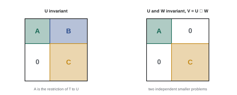
When \(U\) is invariant, the restriction \(T|_U : U \to U\) is an operator in its own right. Choose a basis of \(U\) and extend it to a basis of \(V\). Because the first basis vectors are sent into their own span, the matrix of \(T\) has a block of zeros in the lower left:
The block \(C\) is the matrix of the induced operator on the quotient \(V/U\) from lesson 3. Taking determinants, \(p_T = p_{T|_U} \cdot p_{T/U}\): the characteristic polynomial factors along any invariant subspace. If \(V = U \oplus W\) with both \(U\) and \(W\) invariant, the block \(B\) vanishes too and the matrix is block diagonal. Splitting \(V\) into invariant pieces in this way is the main strategy of the structure theory.
Upper triangular form
Theorem (triangularization). Every operator on a finite-dimensional complex vector space has an upper triangular matrix in some basis. Moreover, the basis can be chosen orthonormal (Schur's theorem).
Proof by induction on \(n = \dim V\). For \(n = 1\) every matrix is triangular. For larger \(n\), \(T\) has an eigenvalue \(\lambda\) (lesson 5); let \(\mathbf{v}_1\) be an eigenvector. The quotient operator on \(V/\operatorname{span}(\mathbf{v}_1)\) acts on a space of dimension \(n - 1\), so by induction it has a triangular matrix in some basis \(\bar{\mathbf{v}}_2, \dots, \bar{\mathbf{v}}_n\). Lift these cosets to vectors \(\mathbf{v}_2, \dots, \mathbf{v}_n\). Then \(T\mathbf{v}_j\) lies in the span of \(\mathbf{v}_1, \dots, \mathbf{v}_j\) for every \(j\), which is what triangular means. For the orthonormal version, replace the quotient by the orthogonal complement of \(\mathbf{v}_1\) and use Gram–Schmidt (lesson 9).
An equivalent statement: \(T\) is triangular in the basis \(\mathbf{v}_1, \dots, \mathbf{v}_n\) exactly when each \(\operatorname{span}(\mathbf{v}_1, \dots, \mathbf{v}_j)\) is invariant. Such a nested chain of invariant subspaces is called a flag. The diagonal entries of a triangular matrix are its eigenvalues, each appearing as often as its algebraic multiplicity, since the determinant of a triangular matrix is the product of its diagonal.
Polynomials in an operator
For a polynomial \(q(x) = c_0 + c_1x + \dots + c_mx^m\), set \(q(T) = c_0I + c_1T + \dots + c_mT^m\). The map \(q \mapsto q(T)\) respects sums and products: \((qr)(T) = q(T)r(T)\). In particular any two polynomials in \(T\) commute. If \(T\mathbf{v} = \lambda\mathbf{v}\) then \(q(T)\mathbf{v} = q(\lambda)\mathbf{v}\), so eigenvectors of \(T\) are eigenvectors of every \(q(T)\).
Because \(L(V)\) has dimension \(n^2\), the \(n^2 + 1\) operators \(I, T, T^2, \dots, T^{n^2}\) must be linearly dependent. So some nonzero polynomial kills \(T\). Among all such polynomials, choose one of least degree and scale it to be monic; this is the minimal polynomial \(m_T\).
Theorem. A polynomial \(q\) satisfies \(q(T) = 0\) exactly when \(m_T\) divides \(q\). Proof: divide, \(q = sm_T + r\) with \(\deg r < \deg m_T\). Then \(r(T) = q(T) - s(T)m_T(T) = q(T)\). If \(q(T) = 0\) then \(r(T) = 0\), and minimality forces \(r = 0\). The converse is immediate. It follows that the minimal polynomial is unique.
Theorem. The roots of \(m_T\) are exactly the eigenvalues of \(T\). Proof: if \(T\mathbf{v} = \lambda\mathbf{v}\) with \(\mathbf{v} \ne \mathbf{0}\), then \(0 = m_T(T)\mathbf{v} = m_T(\lambda)\mathbf{v}\), so \(m_T(\lambda) = 0\). Conversely, if \(m_T(\lambda) = 0\), write \(m_T(x) = (x - \lambda)s(x)\). Since \(\deg s < \deg m_T\), \(s(T) \ne 0\), so some \(\mathbf{w}\) has \(\mathbf{v} = s(T)\mathbf{w} \ne \mathbf{0}\), and \((T - \lambda I)\mathbf{v} = m_T(T)\mathbf{w} = \mathbf{0}\).
The Cayley–Hamilton theorem
Theorem. Every operator satisfies its characteristic polynomial: \(p_T(T) = 0\). Consequently \(m_T\) divides \(p_T\), and \(\deg m_T \le n\), a big improvement on the crude bound \(n^2\).
Proof over \(\mathbb{C}\). Choose a basis \(\mathbf{v}_1, \dots, \mathbf{v}_n\) in which \(T\) is upper triangular with diagonal \(\lambda_1, \dots, \lambda_n\), so \(p_T(x) = (x - \lambda_1)\cdots(x - \lambda_n)\). Let \(V_j = \operatorname{span}(\mathbf{v}_1, \dots, \mathbf{v}_j)\). Triangularity says \((T - \lambda_jI)\mathbf{v}_j \in V_{j-1}\), so \((T - \lambda_jI)V_j \subseteq V_{j-1}\). Applying the factors in turn, \((T - \lambda_1I)\cdots(T - \lambda_nI)V\) lies in \((T - \lambda_1I)\cdots(T - \lambda_{n-1}I)V_{n-1}\), and so on down to \((T - \lambda_1I)V_1 = \{\mathbf{0}\}\). (The factors commute, so their order does not matter.) For real matrices, regard them as complex matrices: the identity \(p_A(A) = 0\) is a statement about the entries and does not care which field we computed in.
A warning about a tempting false proof: substituting \(\lambda = A\) into \(\det(\lambda I - A)\) to get \(\det(A - A) = 0\) confuses a matrix with a scalar. The left side \(p_A(A)\) is a matrix; the 'proof' produces the number 0. The theorem is true, but not for that reason.
Worked problem
Cayley–Hamilton and the inverse
For \(A = \begin{pmatrix} 2 & 1 \\ 1 & 3 \end{pmatrix}\), verify Cayley–Hamilton and use it to find \(A^{-1}\) and \(A^3\).
Show solution
- \(p_A(x) = x^2 - (\operatorname{tr}A)x + \det A = x^2 - 5x + 5\).
- \(A^2 = \begin{pmatrix} 5 & 5 \\ 5 & 10 \end{pmatrix}\), and \(A^2 - 5A + 5I = \begin{pmatrix} 5 - 10 + 5 & 5 - 5 \\ 5 - 5 & 10 - 15 + 5 \end{pmatrix} = 0\).
- Rearranging, \(A(A - 5I) = -5I\), so \(A^{-1} = \frac{1}{5}(5I - A) = \frac{1}{5}\begin{pmatrix} 3 & -1 \\ -1 & 2 \end{pmatrix}\).
- Also \(A^2 = 5A - 5I\), so \(A^3 = 5A^2 - 5A = 5(5A - 5I) - 5A = 20A - 25I = \begin{pmatrix} 15 & 20 \\ 20 & 35 \end{pmatrix}\).
Answer: \(A^{-1} = \frac{1}{5}\begin{pmatrix} 3 & -1 \\ -1 & 2 \end{pmatrix}\) and \(A^3 = 20A - 25I\). Every power of a \(2 \times 2\) matrix is a combination of \(I\) and \(A\).
The minimal polynomial and diagonalizability
Theorem. \(T\) is diagonalizable exactly when \(m_T\) is a product of distinct linear factors, \(m_T(x) = (x - \lambda_1)\cdots(x - \lambda_k)\).
One direction is easy. If \(T\) is diagonalizable with distinct eigenvalues \(\lambda_1, \dots, \lambda_k\), then \((T - \lambda_1I)\cdots(T - \lambda_kI)\) kills every eigenvector (one factor kills it, and the factors commute) and hence kills a basis. So \(m_T\) divides this product of distinct factors; since every eigenvalue is a root of \(m_T\), they are equal.
For the converse, suppose \(m_T = (x - \lambda_1)\cdots(x - \lambda_k)\) with distinct \(\lambda_i\). Use the Lagrange polynomials \(\ell_i(x) = \prod_{j \ne i}(x - \lambda_j)/(\lambda_i - \lambda_j)\), which satisfy \(\ell_1 + \dots + \ell_k = 1\) (a polynomial of degree less than \(k\) that equals 1 at \(k\) points). Then every \(\mathbf{v} = \ell_1(T)\mathbf{v} + \dots + \ell_k(T)\mathbf{v}\), and \((T - \lambda_iI)\ell_i(T)\mathbf{v}\) is a multiple of \(m_T(T)\mathbf{v} = \mathbf{0}\). So each piece is in \(E_{\lambda_i}\) and the eigenspaces span \(V\). The operators \(\ell_i(T)\) are exactly the spectral projections \(\Pi_i\) of lesson 6.
This criterion is often the quickest test. A projection satisfies \(P^2 = P\), so \(m_P\) divides \(x(x - 1)\) and \(P\) is diagonalizable. A reflection satisfies \(R^2 = I\), so \(m_R\) divides \((x - 1)(x + 1)\). Any matrix with \(A^k = I\) over \(\mathbb{C}\) is diagonalizable, because \(x^k - 1\) has \(k\) distinct roots. A nonzero nilpotent matrix has \(m_N = x^r\) with \(r \ge 2\) and is not diagonalizable.
| Operator | Characteristic polynomial | Minimal polynomial | Diagonalizable? |
|---|---|---|---|
| \(I_3\) | \((x - 1)^3\) | \(x - 1\) | Yes |
| \(\begin{pmatrix} 2 & 1 & 0 \\ 0 & 2 & 0 \\ 0 & 0 & 3 \end{pmatrix}\) | \((x - 2)^2(x - 3)\) | \((x - 2)^2(x - 3)\) | No |
| \(\operatorname{diag}(2, 2, 3)\) | \((x - 2)^2(x - 3)\) | \((x - 2)(x - 3)\) | Yes |
| Projection onto a plane in \(\mathbb{R}^3\) | \(x(x - 1)^2\) | \(x(x - 1)\) | Yes |
| \(D\) on \(P_3\) | \(x^4\) | \(x^4\) | No |
The second and third rows have the same characteristic polynomial but different minimal polynomials, so they are not similar. The minimal polynomial sees structure that the characteristic polynomial misses, but even together they are not a complete invariant for matrices of size 4 and larger; the Jordan form is.
Computing the minimal polynomial
A practical way to find \(m_A\) is to look for the first linear dependence among \(I, A, A^2, \dots\), flattened into vectors. By Cayley–Hamilton the search stops by degree \(n\). The code does this with exact fractions for a matrix whose minimal polynomial has lower degree than its characteristic polynomial, then checks Cayley–Hamilton directly.
from fractions import Fraction as F

def mul(X, Y):
    n = len(X)
    return [[sum(X[i][k] * Y[k][j] for k in range(n)) for j in range(n)] for i in range(n)]

def rref_rank(rows):
    M = [r[:] for r in rows]
    r = 0
    for c in range(len(M[0])):
        p = next((i for i in range(r, len(M)) if M[i][c] != 0), None)
        if p is None:
            continue
        M[r], M[p] = M[p], M[r]
        M[r] = [x / M[r][c] for x in M[r]]
        for i in range(len(M)):
            if i != r and M[i][c] != 0:
                M[i] = [a - M[i][c] * b for a, b in zip(M[i], M[r])]
        r += 1
    return r

A = [[F(x) for x in row] for row in [[3, 1, 0, 0], [0, 3, 0, 0], [0, 0, 3, 0], [0, 0, 0, 5]]]
n = len(A)
I = [[F(int(i == j)) for j in range(n)] for i in range(n)]
powers = [I]
while True:
    vecs = [[x for row in P for x in row] for P in powers]
    if rref_rank(vecs) < len(vecs):
        break
    powers.append(mul(powers[-1], A))
print("first dependence among I, A, ..., A^k at k =", len(powers) - 1)

# solve c_0 I + ... + c_(k-1) A^(k-1) = -A^k exactly by Gaussian elimination
k = len(powers) - 1
vecs = [[x for row in P for x in row] for P in powers]
aug = [[vecs[d][e] for d in range(k)] + [-vecs[k][e]] for e in range(n * n)]
r, piv = 0, []
for c in range(k):
    p = next((i for i in range(r, len(aug)) if aug[i][c] != 0), None)
    if p is None:
        continue
    aug[r], aug[p] = aug[p], aug[r]
    aug[r] = [x / aug[r][c] for x in aug[r]]
    for i in range(len(aug)):
        if i != r and aug[i][c] != 0:
            aug[i] = [a - aug[i][c] * b for a, b in zip(aug[i], aug[r])]
    piv.append(c)
    r += 1
coeffs = [aug[piv.index(c)][-1] for c in range(k)]
print("minimal polynomial coefficients (constant term first, monic):", ", ".join(str(c) for c in coeffs + [1]))

# Cayley-Hamilton: p(x) = (x - 3)^3 (x - 5)
M3 = [[A[i][j] - 3 * I[i][j] for j in range(n)] for i in range(n)]
M5 = [[A[i][j] - 5 * I[i][j] for j in range(n)] for i in range(n)]
pA = mul(mul(mul(M3, M3), M3), M5)
print("p_A(A) is zero:", all(x == 0 for row in pA for x in row))
mA = mul(mul(M3, M3), M5)
print("(A - 3I)^2 (A - 5I) is zero:", all(x == 0 for row in mA for x in row))
mB = mul(M3, M5)
print("(A - 3I)(A - 5I) is zero:", all(x == 0 for row in mB for x in row))first dependence among I, A, ..., A^k at k = 3 minimal polynomial coefficients (constant term first, monic): -45, 39, -11, 1 p_A(A) is zero: True (A - 3I)^2 (A - 5I) is zero: True (A - 3I)(A - 5I) is zero: False
The output confirms that the minimal polynomial is \((x - 3)^2(x - 5) = x^3 - 11x^2 + 39x - 45\). The squared factor tells us that \(A\) is not diagonalizable, and that its largest Jordan block for eigenvalue 3 has size 2, as lesson 8 will explain. Finding the coefficients is just solving the linear system given by the first dependence, which is what the elimination step does.
Where this leads
The minimal polynomial factors as \(m_T(x) = (x - \lambda_1)^{r_1}\cdots(x - \lambda_k)^{r_k}\) over \(\mathbb{C}\). The same Lagrange-style argument, using polynomials that are 1 modulo one factor \((x - \lambda_i)^{r_i}\) and 0 modulo the others, splits \(V\) into a direct sum of invariant subspaces \(\ker(T - \lambda_iI)^{r_i}\), the generalized eigenspaces. On each, \(T - \lambda_iI\) is nilpotent. Lesson 8 analyses nilpotent operators completely, and the result is the Jordan canonical form.
Common mistakes
MistakeProving Cayley–Hamilton by substituting \(A\) for \(\lambda\) inside the determinant.
InsteadThat produces the scalar 0, not the zero matrix; use triangularization or the adjugate.
MistakeAssuming the minimal polynomial equals the characteristic polynomial.
InsteadIt divides it and has the same roots, but exponents can be smaller.
MistakeThinking an invariant subspace must be an eigenspace.
InsteadAny span of eigenvectors, any kernel or image of a polynomial in \(T\), and many others are invariant.
MistakeConcluding that a block triangular matrix is block diagonal.
InsteadYou also need an invariant complement for the upper-right block to vanish.
MistakeTesting diagonalizability with the characteristic polynomial alone.
InsteadUse the minimal polynomial: distinct linear factors are needed.
Summary and key terms
- An invariant subspace gives a block triangular matrix, and the characteristic polynomial factors accordingly.
- Every complex operator is upper triangular in some basis, even an orthonormal one.
- The minimal polynomial is the monic polynomial of least degree killing \(T\); it divides every polynomial that kills \(T\).
- Its roots are exactly the eigenvalues.
- Cayley–Hamilton: \(p_T(T) = 0\), so the minimal polynomial divides the characteristic polynomial.
- \(T\) is diagonalizable exactly when its minimal polynomial has distinct linear factors.
- invariant subspace
- A subspace \(U\) with \(T(U) \subseteq U\).
- restriction
- The operator \(T|_U\) on an invariant subspace.
- flag
- A nested chain of subspaces of dimensions 1, 2, ..., n.
- minimal polynomial
- The monic polynomial of least degree with \(m(T) = 0\).
- Cayley–Hamilton theorem
- Every operator satisfies its own characteristic polynomial.
- generalized eigenspace
- \(\ker(T - \lambda I)^{r}\) for large enough \(r\).
- triangularization
- Choosing a basis in which the matrix is upper triangular.
- annihilating polynomial
- Any polynomial \(q\) with \(q(T) = 0\).
Practice problems
Work each problem on paper first, then reveal the answer to check.
Prove that \(\ker T\) and \(\operatorname{im} T\) are invariant under \(T\).
Show answer
If \(T\mathbf{v} = 0\) then \(T(T\mathbf{v}) = 0\); and \(T(T\mathbf{w}) \in \operatorname{im}T\).
Prove that if \(ST = TS\), then every eigenspace of \(T\) is invariant under \(S\).
Show answer
If \(T\mathbf{v} = \lambda\mathbf{v}\) then \(T(S\mathbf{v}) = S(T\mathbf{v}) = \lambda S\mathbf{v}\).
Find the minimal polynomial of \(\begin{pmatrix} 0 & 1 \\ -1 & 0 \end{pmatrix}\).
Show answer
\(x^2 + 1\), since the matrix squares to \(-I\) and is not a scalar multiple of \(I\).
Use Cayley–Hamilton to express \(A^{-1}\) as a polynomial in \(A\) when \(p_A(x) = x^3 - 2x^2 + x - 4\).
Show answer
\(A^3 - 2A^2 + A = 4I\), so \(A^{-1} = \frac{1}{4}(A^2 - 2A + I)\).
Prove that a matrix with \(A^3 = A\) is diagonalizable over \(\mathbb{R}\).
Show answer
\(m_A\) divides \(x^3 - x = x(x - 1)(x + 1)\), which has distinct real roots.
Show that a \(3 \times 3\) nilpotent matrix satisfies \(N^3 = 0\).
Show answer
Its characteristic polynomial is \(x^3\) (only eigenvalue 0), so Cayley–Hamilton gives \(N^3 = 0\).
Lesson quiz · 5 questions
Score 60% or more to complete this lesson.
Create a free account to save your progress, take quizzes and earn a certificate.