
MATH-221 · Lesson 4 of 12 · 22 min
Matrices of linear maps and change of basis
Lesson 3 treated linear maps abstractly. To compute with them we need numbers, and numbers come from bases. Once you choose a basis for the domain and a basis for the codomain, every linear map becomes a matrix, every vector becomes a column, and applying the map becomes matrix multiplication. Choosing different bases gives a different matrix for the same map. This lesson builds the matrix of a linear map, shows how it changes when the bases change, and introduces similarity, the relation between two matrices that describe the same operator in different coordinates. The rest of the course, from diagonalization to the singular value decomposition, is a search for the basis in which a map's matrix is as simple as possible.
The matrix of a linear map
Let \(T : V \to W\) be linear, with ordered basis \(\mathcal{B} = (\mathbf{b}_1, \dots, \mathbf{b}_n)\) for \(V\) and \(\mathcal{C} = (\mathbf{c}_1, \dots, \mathbf{c}_m)\) for \(W\). Because \(T\) is determined by its values on a basis, record those values in coordinates. The matrix of \(T\) relative to \(\mathcal{B}\) and \(\mathcal{C}\) is the \(m \times n\) matrix whose \(j\)th column is the \(\mathcal{C}\)-coordinate vector of \(T(\mathbf{b}_j)\):
The defining property is that the matrix does in coordinates what \(T\) does to vectors:
Proof: write \(\mathbf{v} = x_1\mathbf{b}_1 + \dots + x_n\mathbf{b}_n\). Then \(T(\mathbf{v}) = x_1T(\mathbf{b}_1) + \dots + x_nT(\mathbf{b}_n)\), and taking coordinates (a linear operation) gives \(x_1\) times column 1 plus ... plus \(x_n\) times column \(n\), which is the matrix times the column \((x_1, \dots, x_n)\). The notation \(\mathcal{C} \gets \mathcal{B}\) reads right to left, like the multiplication: feed in \(\mathcal{B}\)-coordinates, get out \(\mathcal{C}\)-coordinates.
For an operator \(T : V \to V\) we usually use the same basis on both sides and write \([T]_{\mathcal{B}}\). When \(V = \mathbb{R}^n\) and \(\mathcal{B}\) is the standard basis, \([T]_{\mathcal{B}}\) is the standard matrix you met in MATH-125.
Worked problem
The derivative as a matrix
Find the matrix of \(D : P_3 \to P_3\), \(D(p) = p\prime\), in the standard basis \(\mathcal{B} = (1, t, t^2, t^3)\), and use it to differentiate \(p = 5 - 2t + 3t^2 + t^3\).
Show solution
- Apply \(D\) to each basis vector: \(D(1) = 0\), \(D(t) = 1\), \(D(t^2) = 2t\), \(D(t^3) = 3t^2\).
- Their coordinate vectors are \((0, 0, 0, 0)\), \((1, 0, 0, 0)\), \((0, 2, 0, 0)\), \((0, 0, 3, 0)\); these are the columns.
- So \([D]_{\mathcal{B}} = \begin{pmatrix} 0 & 1 & 0 & 0 \\ 0 & 0 & 2 & 0 \\ 0 & 0 & 0 & 3 \\ 0 & 0 & 0 & 0 \end{pmatrix}\).
- With \([p]_{\mathcal{B}} = (5, -2, 3, 1)\), the product is \((-2, 6, 3, 0)\), which is \(-2 + 6t + 3t^2\). That is indeed \(p\prime\).
Answer: \([D]_{\mathcal{B}}\) has the entries 1, 2, 3 just above the diagonal and zeros elsewhere; \(p\prime = -2 + 6t + 3t^2\).
Observe that \([D]_{\mathcal{B}}\) is strictly upper triangular and \(D^4 = 0\): differentiating a cubic four times gives zero. Such operators are called nilpotent, and they reappear in lesson 8 as the building blocks of the Jordan form.
Composition is multiplication
If \(T : U \to V\) and \(S : V \to W\) with bases \(\mathcal{A}, \mathcal{B}, \mathcal{C}\), then
Proof: apply both sides to \([\mathbf{u}]_{\mathcal{A}}\) and use the defining property twice. The inner subscripts \(\mathcal{B}\) cancel, like a chain. This identity is the real reason matrix multiplication is defined row by column: it is the unique definition that makes composing maps correspond to multiplying matrices. Associativity of matrix multiplication follows for free from associativity of composition, with no index juggling.
Similarly, \([S + T] = [S] + [T]\) and \([cT] = c[T]\). Together these say that the map \(T \mapsto [T]_{\mathcal{C} \gets \mathcal{B}}\) is an isomorphism from \(L(V, W)\) to \(M_{m \times n}\), so \(\dim L(V, W) = \dim V \cdot \dim W\).
Change of basis for vectors
Suppose \(\mathcal{B}\) and \(\mathcal{B}'\) are two bases of the same space \(V\). The change-of-coordinates matrix from \(\mathcal{B}\) to \(\mathcal{B}'\) is the matrix of the identity map with \(\mathcal{B}\) on the input side and \(\mathcal{B}'\) on the output side:
Its columns are the old basis vectors written in the new basis. It is invertible, and its inverse goes the other way: \(P_{\mathcal{B} \gets \mathcal{B}'} = (P_{\mathcal{B}' \gets \mathcal{B}})^{-1}\). In \(\mathbb{R}^n\), if \(\mathcal{E}\) is the standard basis, then \(P_{\mathcal{E} \gets \mathcal{B}}\) is simply the matrix whose columns are the vectors of \(\mathcal{B}\), and \(P_{\mathcal{B} \gets \mathcal{E}}\) is its inverse. To go between two non-standard bases, route through the standard one: \(P_{\mathcal{B}' \gets \mathcal{B}} = P_{\mathcal{B}' \gets \mathcal{E}} P_{\mathcal{E} \gets \mathcal{B}}\).
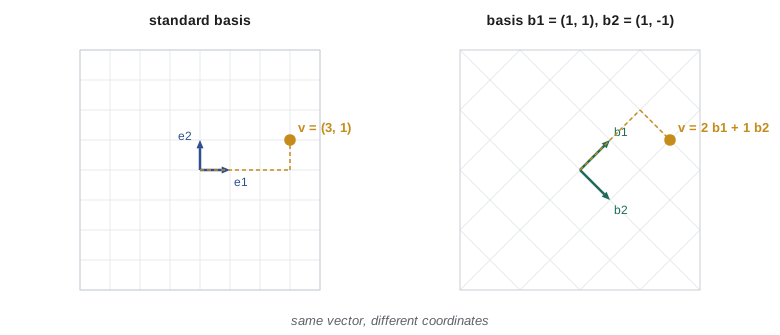
A common confusion is direction. The matrix whose columns are the new basis vectors converts new coordinates into standard coordinates, not the other way round. When in doubt, test it on one basis vector: the first new basis vector has new coordinates \((1, 0, \dots, 0)\), and the matrix should turn that into its standard coordinates.
Change of basis for operators and similarity
Now let \(T : V \to V\) be an operator with matrices \(A = [T]_{\mathcal{B}}\) and \(A' = [T]_{\mathcal{B}'}\). To compute \(A'\) applied to new coordinates, convert to old coordinates, apply \(A\), then convert back:
Two square matrices \(A\) and \(A'\) are similar if \(A' = P^{-1}AP\) for some invertible \(P\). Similar matrices are the same linear operator seen in two coordinate systems. Anything that describes the operator rather than the coordinates must therefore be the same for similar matrices. Such quantities are called similarity invariants:
| Invariant | Why it is the same for similar matrices |
|---|---|
| Determinant | \(\det(P^{-1}AP) = \det(P)^{-1}\det A \det P = \det A\) |
| Trace | \(\operatorname{tr}(XY) = \operatorname{tr}(YX)\), so \(\operatorname{tr}(P^{-1}(AP)) = \operatorname{tr}((AP)P^{-1})\) |
| Rank | Multiplying by invertible matrices does not change the dimension of the image |
| Characteristic polynomial | \(\det(P^{-1}AP - \lambda I) = \det(P^{-1}(A - \lambda I)P)\) |
| Eigenvalues | They are the roots of the characteristic polynomial |
| Minimal polynomial | \(q(P^{-1}AP) = P^{-1}q(A)P\) for any polynomial \(q\) |
These invariants let you tell quickly when two matrices cannot be similar: different traces or determinants settle it. The converse is harder. Two matrices can share trace, determinant and characteristic polynomial without being similar; \(I\) and \(\begin{pmatrix} 1 & 1 \\ 0 & 1 \end{pmatrix}\) are the standard example. Lesson 8 shows that the Jordan form is a complete invariant: two matrices are similar exactly when they have the same Jordan form.
A worked change of basis
Take the operator on \(\mathbb{R}^2\) with standard matrix \(A = \begin{pmatrix} 2 & 1 \\ 1 & 2 \end{pmatrix}\) and the basis \(\mathcal{B}' = (\mathbf{b}_1, \mathbf{b}_2)\) with \(\mathbf{b}_1 = (1, 1)\), \(\mathbf{b}_2 = (1, -1)\). Here \(P = \begin{pmatrix} 1 & 1 \\ 1 & -1 \end{pmatrix}\), whose columns are the new basis vectors. The code computes \(P^{-1}AP\) exactly and also converts a vector's coordinates both ways.
from fractions import Fraction as F

def mul(X, Y):
    return [[sum(X[i][k] * Y[k][j] for k in range(len(Y))) for j in range(len(Y[0]))] for i in range(len(X))]

def inv2(M):
    (a, b), (c, d) = M
    det = F(a * d - b * c)
    return [[d / det, -b / det], [-c / det, a / det]]

A = [[2, 1], [1, 2]]
P = [[1, 1], [1, -1]]           # columns are b1 = (1, 1) and b2 = (1, -1)
Pinv = inv2(P)
Anew = mul(mul(Pinv, A), P)
print("matrix of T in the new basis:", [[str(x) for x in row] for row in Anew])

v_std = [[3], [1]]              # standard coordinates of v
v_new = mul(Pinv, v_std)
print("new coordinates of (3, 1):", [str(r[0]) for r in v_new])
back = mul(P, v_new)
print("converted back to standard:", [str(r[0]) for r in back])
print("trace and determinant unchanged:",
      A[0][0] + A[1][1], Anew[0][0] + Anew[1][1], "|",
A[0][0] * A[1][1] - A[0][1] * A[1][0], Anew[0][0] * Anew[1][1] - Anew[0][1] * Anew[1][0])matrix of T in the new basis: [['3', '0'], ['0', '1']] new coordinates of (3, 1): ['2', '1'] converted back to standard: ['3', '1'] trace and determinant unchanged: 4 4 | 3 3
In the new basis the matrix is diagonal, with entries 3 and 1. That is no accident: \(\mathbf{b}_1\) and \(\mathbf{b}_2\) are eigenvectors of \(A\), with eigenvalues 3 and 1. In the eigenvector basis the operator simply stretches each axis. Lesson 6 develops this into diagonalization; the point here is that the right basis can turn a full matrix into a diagonal one without changing the operator at all.
Changing bases in both spaces
For a map \(T : V \to W\) between different spaces, we may change the basis on each side independently. If \(P\) changes coordinates in \(V\) and \(Q\) changes coordinates in \(W\), then the new matrix is \(Q^{-1}AP\). Because the two changes are independent, we have far more freedom than for operators, and the simplest possible form is very simple indeed.
Theorem (rank normal form). If \(T : V \to W\) has rank \(r\), there are bases of \(V\) and \(W\) in which the matrix of \(T\) has the \(r \times r\) identity in its top-left corner and zeros everywhere else. Proof sketch: choose a basis of \(V\) whose last \(n - r\) vectors span the kernel (as in the proof of rank–nullity); the images of the first \(r\) vectors are independent, so extend them to a basis of \(W\). In these bases, the first \(r\) basis vectors go to the first \(r\) basis vectors and the rest go to zero.
So, up to a choice of bases on both sides, the only thing a linear map has is its rank. For operators, where we must use one basis on both sides, the story is much richer, and that richness, captured by eigenvalues and the Jordan form, occupies lessons 6 to 8. The singular value decomposition of lesson 12 is a version of rank normal form in which both bases are required to be orthonormal; then the identity block becomes a diagonal block of singular values.
Polynomial spaces and other bases
Change of basis is not only about \(\mathbb{R}^n\). In \(P_2\), the standard basis is \((1, t, t^2)\), but for interpolation the Lagrange basis built on nodes \(0, 1, 2\) is often better: its vectors are the quadratics that equal 1 at one node and 0 at the others. The coordinates of a polynomial in the Lagrange basis are simply its values at the nodes. The change-of-basis matrix from Lagrange coordinates to standard coordinates has as columns the coefficients of the Lagrange polynomials, and its inverse is the Vandermonde matrix of the nodes. Numerical analysts choose among the standard, Lagrange, Newton, Chebyshev and Bernstein bases according to which makes their computation stable; computer graphics uses the Bernstein basis because its coordinates are the control points of a Bézier curve.
Common mistakes
MistakePutting \(T(\mathbf{b}_j)\) in the rows of the matrix.
InsteadThe coordinates of \(T(\mathbf{b}_j)\) form the \(j\)th column.
MistakeUsing the matrix of new basis vectors to convert standard coordinates into new ones.
InsteadThat matrix converts new coordinates into standard ones; use its inverse for the other direction.
MistakeWriting \(PAP^{-1}\) when you mean \(P^{-1}AP\).
InsteadWith \(P = P_{\mathcal{B} \gets \mathcal{B}\prime}\), the new matrix is \(P^{-1}AP\); check by applying it to a new basis vector.
MistakeConcluding two matrices are similar because they have the same eigenvalues.
InsteadEqual invariants are necessary but not sufficient; compare Jordan forms.
MistakeForgetting that coordinates depend on the order of the basis.
InsteadPermuting the basis permutes the rows and columns of the matrix.
Summary and key terms
- The matrix of \(T\) relative to bases \(\mathcal{B}, \mathcal{C}\) has columns \([T(\mathbf{b}_j)]_{\mathcal{C}}\), and \([T\mathbf{v}]_{\mathcal{C}} = [T][\mathbf{v}]_{\mathcal{B}}\).
- Composition of maps corresponds to multiplication of their matrices, which explains the definition of matrix multiplication.
- A change-of-coordinates matrix has the old basis vectors, written in the new basis, as its columns.
- For an operator, a change of basis replaces \(A\) by \(P^{-1}AP\); such matrices are similar.
- Determinant, trace, rank, characteristic polynomial and eigenvalues are similarity invariants.
- With independent bases on both sides, every map has the rank normal form; for operators the right basis is the subject of the next lessons.
- matrix of a linear map
- The matrix whose columns are the coordinates of the images of the domain basis.
- change-of-coordinates matrix
- The matrix that converts coordinates in one basis into coordinates in another.
- similar matrices
- Matrices with \(A\prime = P^{-1}AP\) for some invertible \(P\).
- similarity invariant
- A quantity that is the same for all similar matrices.
- nilpotent operator
- An operator with \(N^k = 0\) for some \(k\).
- rank normal form
- The block form with an identity of size equal to the rank and zeros elsewhere.
- Lagrange basis
- Polynomials that equal 1 at one interpolation node and 0 at the others.
- standard matrix
- The matrix of a map between coordinate spaces in the standard bases.
Practice problems
Work each problem on paper first, then reveal the answer to check.
Find the matrix of the transpose operator on \(M_{2 \times 2}\) in the basis \(E_{11}, E_{12}, E_{21}, E_{22}\).
Show answer
It swaps the second and third basis vectors: the permutation matrix with rows \((1,0,0,0), (0,0,1,0), (0,1,0,0), (0,0,0,1)\).
If \(\mathcal{B} = ((1, 2), (3, 7))\), find \([\mathbf{v}]_{\mathcal{B}}\) for \(\mathbf{v} = (1, 0)\).
Show answer
\(P = \begin{pmatrix} 1 & 3 \\ 2 & 7 \end{pmatrix}\), \(P^{-1} = \begin{pmatrix} 7 & -3 \\ -2 & 1 \end{pmatrix}\), so the coordinates are \((7, -2)\).
Prove that similar matrices have the same trace.
Show answer
\(\operatorname{tr}(P^{-1}AP) = \operatorname{tr}(APP^{-1}) = \operatorname{tr}A\) using \(\operatorname{tr}(XY) = \operatorname{tr}(YX)\).
Explain why \(\begin{pmatrix} 1 & 2 \\ 3 & 4 \end{pmatrix}\) and \(\begin{pmatrix} 1 & 0 \\ 0 & 4 \end{pmatrix}\) are not similar.
Show answer
Their traces are 5 and 5 but their determinants are \(-2\) and 4.
Show that if \(A\) is similar to \(I\) then \(A = I\).
Show answer
\(A = P^{-1}IP = I\).
What is \(\dim L(P_2, M_{2 \times 2})\)?
Show answer
\(3 \times 4 = 12\).
Lesson quiz · 5 questions
Score 60% or more to complete this lesson.
Create a free account to save your progress, take quizzes and earn a certificate.